Robust principal component analysis: Definition & Examples

Robust principal component analysis (robust PCA) seeks low-dimensional structure while resisting contamination that can distort ordinary PCA. In the low-rank-plus-sparse formulation developed here, a quant models a data panel as a common component plus a small number of potentially large entry-level disturbances. A bad quote in one instrument on one date need not define the fitted common movement.

“Robust PCA” covers several approaches. This article focuses on principal component pursuit (PCP), the convex decomposition studied by Candès, Li, Ma and Wright, rather than treating that name as a synonym for every robust subspace estimator.

Two structures, two penalties

For an observed matrix $M\in\mathbb{R}^{m\times n}$ , the idealised model is

M=L_0+S_0.

The matrix rank of

L_0

is small; most entries of

S_0

are zero. The nonzero disturbances need not be small. PCP estimates both matrices through

\min_{L,S}\;\lVert L\rVert_*+\lambda\lVert S\rVert_1 \quad\text{subject to}\quad L+S=M,\qquad \lambda>0.

Here

\lVert L\rVert_*=\sum_j\sigma_j(L)

is the nuclear norm, the sum of singular values. The entrywise norm is

\lVert S\rVert_1=\sum_{i,j}|S_{ij}|

, not the maximum absolute column sum sometimes called the matrix 1-norm. These convex penalties favour low rank and sparse entries respectively. Increasing

\lambda

makes assigning magnitude to

S

more expensive relative to assigning it to

L

This differs from an ordinary low-rank approximation, which compresses the observed matrix without explicitly separating sparse corruption. The stable PCP paper explains why sparse gross errors and small, widespread perturbations require different treatment.

A decomposition you can audit by hand

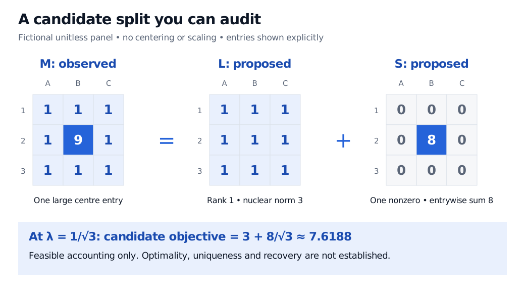
Consider a fictional, unitless three-by-three panel, with no centering or scaling applied:

M=\begin{pmatrix}1&1&1\\1&9&1\\1&1&1\end{pmatrix},\qquad L=\begin{pmatrix}1&1&1\\1&1&1\\1&1&1\end{pmatrix},\qquad S=\begin{pmatrix}0&0&0\\0&8&0\\0&0&0\end{pmatrix}.

The proposed components sum exactly to $M$ . All columns of $L$ are identical, so its rank is one. Writing $L=\mathbf{1}\mathbf{1}^{\top}$ gives its only nonzero singular value as $\lVert\mathbf{1}\rVert_2^2=3$ . Thus

\lVert L\rVert_*=3,\qquad \lVert S\rVert_1=8.

With $\lambda=1/\sqrt{3}$ , the objective at this candidate is

3+\frac{8}{\sqrt{3}}\approx7.6188.

Fictional unitless three-by-three panel M has centre entry 9 and all other entries 1. The candidate L has nine entries equal to 1 and rank 1; S has centre entry 8 and all other entries zero. They sum exactly to M. The candidate objective at lambda 1 over square root 3 is 7.6188; no optimality or recovery result is asserted.

Original deterministic accounting example. The proposed split has nuclear norm 3 and entrywise absolute sum 8; the diagram does not show an optimisation result.

This establishes feasibility and objective accounting only. It does not establish that PCP selects this split, that the split is unique, or that the centre entry was a data error. Choosing the familiar theoretical weight does not supply those missing conclusions.

Why sparse is not enough

Separation is ambiguous when a component can be both low rank and sparse. A matrix with just one nonzero entry already has rank one: its value could be assigned to either component without changing their sum.

The original PCP recovery theorem therefore requires more than a small corruption count: sufficiently low rank, incoherence of the low-rank singular vectors, and a sufficiently sparse support sampled uniformly among supports of its size. Incoherence prevents the low-rank structure from concentrating on a few coordinates. These are qualifications on a recovery theorem, not diagnostics automatically certified by running an optimiser. The theorem's rectangular weight

1/\sqrt{\max(m,n)}

is justified within its assumptions. See §§1.3–1.4 of the original paper.

For a returns panel, a whole stress date affecting many assets may violate the intended entry-sparse contamination model. It may also be economically meaningful. A large fitted sparse component is a model allocation, not proof that an observation should be deleted from risk analysis.

Noise, covariance and preprocessing

Small noise at most entries is dense, even when each entry is tiny. Stable PCP instead allows

M=L_0+S_0+N_0,\qquad \min_{L,S}\;\lVert L\rVert_*+\lambda\lVert S\rVert_1 \quad\text{subject to}\quad \lVert M-L-S\rVert_F\leq\delta.

The Frobenius norm aggregates squared residual entries, and

\delta

specifies a noise budget. Zhou and co-authors, §I-A, prove a conditional stability result for this relaxation; allowing a residual does not remove the structural assumptions.

Robust covariance estimation targets an outlier-resistant scatter matrix, as described in the official scikit-learn guide. For example, the minimum covariance determinant estimator uses a subset of observation vectors. Diagonalising a robust scatter estimate is a different route to robust directions; it does not produce the PCP entrywise split

M=L+S

Preprocessing belongs to the model specification. Subtracting an ordinary column mean can spread one contaminated cell across a column; changing units changes both penalties. State the panel orientation, units, location treatment and scaling before interpreting components. The toy matrix above is an additive decomposition, not an example of centered covariance PCA.

For the linear foundation, the SelfMadeQuant lesson Principal Component Analysis and the SVD View derives the maximum-variance direction and explains centering and scale. It offers a public preview; the full lesson requires membership.

Sources

Candès, Li, Ma and Wright, Robust Principal Component Analysis?, §§1.1–1.4: formulation, norm conventions, identifiability and conditional exact recovery.
Zhou, Li, Wright, Candès and Ma, Stable Principal Component Pursuit, Introduction and §I-A: dense perturbations, residual-constrained formulation and conditional stability.
scikit-learn, Covariance estimation, §2.6.4: robust scatter estimation and outlier sensitivity.

Two structures, two penalties

A decomposition you can audit by hand

Why sparse is not enough

Noise, covariance and preprocessing

Sources

Related terms

Matrix rank

Minimum covariance determinant estimator

Singular value