A rational function is a ratio of two polynomials:
The denominator polynomial must not be identically zero. For a real-valued function given by this expression, its natural domain contains every real input except the zeros of the original denominator. A model may impose further restrictions. The word rational refers to the ratio of polynomials; its coefficients and outputs need not be rational numbers. A polynomial is itself a rational function, since it can be written over the constant denominator .
A fixed trading charge becomes a curved average cost
Suppose a synthetic execution-fee schedule charges USD 10 per order plus USD 0.05 per share. This is an assumed schedule for teaching, not a broker quote. Let be the number of shares bought. The total fee, measured in USD, is
For a positive order quantity, the average fee per share is the rational function
The USD 10 is the fixed total fee. It becomes the quantity-dependent contribution USD per share only after division. Confusing those units would obscure the entire effect.
| Order quantity | Total fee, USD | Average fee, USD/share |
|---|---|---|
| 100 shares | 15 | 0.15 |
| 1,000 shares | 60 | 0.06 |
A larger order costs more in total while costing less per share. The curve captures the dilution of the fixed charge; the marginal per-share charge remains USD 0.05 under this schedule.
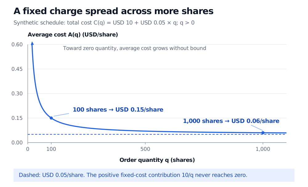
Original synthetic fee model, shown for positive quantities. The curve continues beyond the plotted window; the dashed line is a limiting average cost, not an attained value.
For every finite positive quantity, , so
Thus the horizontal asymptote is USD 0.05 per share, approached from above and never reached at a finite positive quantity. This conclusion follows from this particular formula. Horizontal asymptotes in general can be crossed.
There are two different domain decisions here. Algebra permits every real . The economic story permits only ; if orders must be in whole shares, it permits only positive integers. The smooth curve is a continuous extension useful for understanding the schedule. In that extension, as , because a fixed total charge is being divided by a quantity tending to zero. A zero-share average is undefined, and negative quantities have no meaning in this purchase-order example.
The falling curve alone does not establish an optimal trade size. Spreads, market impact, liquidity, inventory risk and changing fee tiers are absent. Similarly, a rational curve fitted to market observations does not make its asymptote an economic law: its extrapolation remains subject to model risk.
Cancellation can reveal a hole without filling it
Consider the purely algebraic example
The simplification tells us the function agrees with the line away from . It does not supply : the original expression is there. The graph has a removable hole at . Defining a new function with the additional value would fill that hole and give a continuous extension. It is an extra definition, rather than a consequence of cancellation.
A pole, by contrast, is an excluded input at which the rational function grows without bound in magnitude as the input approaches it. It produces a vertical asymptote. The average-cost expression has a pole at . To distinguish holes from poles, factor and cancel all common factors before inspecting the remaining denominator. Merely finding a common factor is insufficient:
One denominator factor remains, so is still a pole. These distinctions are developed in OpenStax's treatment of rational functions.
For a broader foundation in function families and domains, see The Four Representations of a Function and Mathematical Models. For calculating rational-function limits by comparing leading powers, continue with Limits at Infinity, Horizontal Asymptotes, and Asymptotic Comparison. Both offer public previews; their full lessons require membership.
Sources
- James Stewart, Single Variable Calculus: Early Transcendentals, 6th edition, §1.2, “Mathematical Models: A Catalog of Essential Functions,” especially “Rational Functions.”
- OpenStax, Precalculus 2e, §3.7, “Rational Functions” — rational functions, domains, asymptotes and removable discontinuities. The fee schedule and numerical examples here are original.