Random-matrix covariance denoising: Definition & Examples

Random-matrix covariance denoising uses the eigenvalue spectrum predicted by a random-data model to guide the cleaning of an estimated covariance or correlation matrix. The practical aim is to stop sampling noise from masquerading as reliable portfolio risk structure, especially in low-variance directions that an optimiser may exploit.

The method has two separate decisions: which sample modes are compatible with the noise model, and what estimates should replace them? The Marchenko–Pastur law supplies a benchmark for the first decision. Covariance eigenvalue clipping is one possible answer to the second. Random-matrix methods also motivate more refined estimators; denoising is not synonymous with one clipping recipe.

Why a noise spectrum is already spread out

For a clean reference, take a $T\times N$ matrix $X$ with iid entries, known mean zero and variance one. Its population covariance is the identity. Use

S=\frac{1}{T}X^\top X, \qquad q=\frac{N}{T}.

As $N,T\to\infty$ with $q\in(0,1)$ fixed, the limiting sample-eigenvalue bulk has edges

\lambda_-=(1-\sqrt q)^2, \qquad \lambda_+=(1+\sqrt q)^2.

For the analytic reference

N=100

T=400

q=0.25

, these are

0.25

and

2.25

. Population variance is still one in every unit direction: the spread is in the sample estimates. Laloux and colleagues set out this independent-return benchmark and its portfolio motivation.

These numbers use divisor

T

and a known zero mean. If means are estimated, ordinary sample covariance instead centres the columns and divides by

T-1

. For iid Gaussian rows, the corresponding reference has

T-1

degrees of freedom, so its aspect ratio is

N/(T-1)

. Such conventions must be settled before fitting a band.

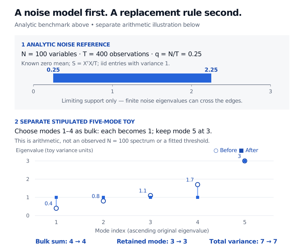
The edges are not hard finite-sample signal tests. Pure noise can produce eigenvalues beyond them. Conversely, agreement with the bulk density alone does not prove that its modes contain no useful structure. Plerou and colleagues explicitly examine finite-size controls and additional spectral tests.

A separate five-mode calculation

Now leave the 100-variable reference behind. Consider an independent, stipulated five-dimensional covariance example, in arbitrary common squared units, with eigenvalues

(0.4,\ 0.8,\ 1.1,\ 1.7,\ 3).

Designate the first four modes as the bulk for this calculation only. Their mean is

\bar\lambda_B=\frac{0.4+0.8+1.1+1.7}{4}=1.

Replacing those four by their mean and retaining the fifth produces $(1,1,1,1,3)$ . Both spectra sum to $7$ . This example demonstrates the transformation; it neither fits a random-matrix model nor establishes that the fifth mode is a genuine factor.

Two separate examples: the analytic iid unit-variance reference for 100 variables and 400 observations has limiting edges 0.25 and 2.25. A stipulated five-mode spectrum 0.4, 0.8, 1.1, 1.7, 3 becomes 1, 1, 1, 1, 3. The selected bulk mean is 1 and both traces are 7.

Original analytic reference and separate arithmetic illustration. The blue band is asymptotic support, not a finite-sample acceptance region. The five modes are stipulated, with bulk membership supplied; no return data or simulation is shown.

Using the eigenvalue decomposition, write

S=U\operatorname{diag}(\lambda_i)U^\top

. For a selected bulk

B

, the averaging rule is

\widetilde S=U\operatorname{diag}(d_i)U^\top, \qquad d_i=\begin{cases} \bar\lambda_B,&i\in B,\\ \lambda_i,&i\notin B. \end{cases}

It retains the sample eigenbasis and preserves trace at this clipping step. In the toy, the spectral condition number falls from

3/0.4=7.5

3/1=3

. That improves this matrix's conditioning; it does not establish more accurate future risk. Bun, Bouchaud and Potters describe bulk averaging and warn that retaining outliers unchanged leaves their estimation error untreated.

When the selected bulk mean is positive, averaging retains residual variance instead of discarding those directions. The relevant distinction is estimation of risk versus low-rank reconstruction. PCA and Factor Compression develops the reconstruction side; its public page is a preview and the full lesson requires membership.

What a usable cleaning procedure still needs

A white-noise reference is a model, not a property of returns. Serial dependence, changing or shared volatility, heavy-tailed observations and genuine cross-asset correlations can change the appropriate benchmark or finite-sample extremes. Heavy tails do not automatically invalidate the bulk law: moment assumptions and the dependence structure matter. A large market mode also absorbs variance, so fitting the residual bulk need not use the unit noise variance of the identity reference. Bouchaud and Potters discuss these return-model complications and the dependence of cleaning performance on the evaluation task.

Cleaning a correlation matrix adds a constraint. Spectral averaging need not preserve its unit diagonal. With positive cleaned diagonal entries, a common rescaling is

D=\operatorname{diag}(\widetilde C_{11},\ldots,\widetilde C_{NN}), \qquad C_{\mathrm{clean}}=D^{-1/2}\widetilde C D^{-1/2}.

This preserves positive semidefiniteness but generally changes the clipped eigenvalues and eigenvectors. Its trace is $N$ because its diagonal is one; do not carry the toy covariance's trace- $7$ claim into a later rescaling. If cleaning correlations, recover covariance with the chosen asset volatilities as $V C_{\mathrm{clean}}V$ , where $V$ is diagonal.

Finally, choose the window, bulk rule and cleaning settings using training data, then assess later risk estimates or portfolio behaviour. A smoother spectrum alone cannot demonstrate improvement. For the risk interpretation behind this check, Eigenvalues and Covariance Matrices derives variance along eigenportfolio directions. The preview is public; the full lesson requires membership.

Sources

Laloux, L., Cizeau, P., Bouchaud, J.-P. and Potters, M. (1999), Noise Dressing of Financial Correlation Matrices, equations (1)–(3) and the finite-size discussion.
Plerou, V. et al. (2002), Random matrix approach to cross correlations in financial data, §§IV–V.
Bun, J., Bouchaud, J.-P. and Potters, M. (2016), Cleaning correlation matrices, “Five cleaning recipes,” equation (5).
Bouchaud, J.-P. and Potters, M. (2009), Financial Applications of Random Matrix Theory: a short review, §§II.A–B and V.B.

Why a noise spectrum is already spread out

A separate five-mode calculation

What a usable cleaning procedure still needs

Sources

Related terms

Covariance eigenvalue clipping

Eigenvalue decomposition

Marchenko–Pastur law

Sample covariance