Rademacher complexity: Definition & Examples

Rademacher complexity measures how well a class of functions can align with random signs. For a quant comparing prediction models, it formalises a capacity concern behind overfitting: a flexible class can make noise look like a pattern. It measures a class on a sample, rather than the performance of one fitted trading strategy.

Hold the observations fixed

For a nonempty real-valued function class $\mathcal F$ and observed inputs $S=(x_1,\ldots,x_n)$ , use the convention

\widehat{\mathcal R}_S(\mathcal F) =\mathbb E_{\sigma}\left[ \sup_{f\in\mathcal F}\frac1n\sum_{i=1}^n\sigma_i f(x_i) \right].

Each

\sigma_i

independently equals

+1

-1

with probability

1/2

, independently of the data. These are artificial random signs, not the observed target labels or market returns. Hold

S

fixed, find the largest signed average within the class for each sign draw, then average over signs. This is the empirical complexity, conditional on the inputs. Cornell's lecture notes use this normalisation.

Expected Rademacher complexity also averages over a fresh random sample from an input distribution $P$ :

\mathcal R_n(\mathcal F) =\mathbb E_{S\sim P^n}\left[\widehat{\mathcal R}_S(\mathcal F)\right].

The empirical quantity can depend on the locations of the observed inputs; the expected quantity depends on their sampling distribution. Neither is simply the number of model parameters.

Two functions are enough to expose the order

Take the deliberately small class containing only $f_+(x)=1$ and $f_-(x)=-1$ . On any two observations,

\sup_{f\in\mathcal F}\frac{\sigma_1 f(x_1)+\sigma_2 f(x_2)}2 =\frac{\lvert\sigma_1+\sigma_2\rvert}{2}.

The class can choose one constant for a whole row. It cannot choose a different function separately for each observation.

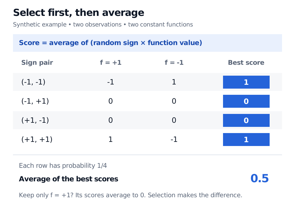
Two constant functions, plus one and minus one, on two observations. The four equally likely random sign pairs give best scores 1, 0, 0, 1 and empirical Rademacher complexity 0.5. A fixed plus-one function has average score zero.

Exact synthetic enumeration: maximise over the two functions separately in each row, then average the four best scores.

Thus the empirical complexity is $(1+0+0+1)/4=0.5$ . Opposite signs cancel because both functions are constant. A class able to realise every sign pattern on two distinct inputs would instead attain score $1$ in every row.

For either constant function fixed before seeing the signs, the expected signed score is zero. Moving the supremum outside the expectation therefore changes the answer. The positive complexity records the class's ability to select a function in response to noise.

This example happens not to depend on the input values, but it still depends on sample size: the same constant class has complexity $1$ at $n=1$ and $3/8$ at $n=4$ . More observations do not give this class more independent choices.

Check the convention before comparing numbers

Some definitions put an absolute value around the signed sum, a factor

2

before

1/n

, or both. Bartlett and Mendelson's original paper, Definition 2, uses both.

Our two-function class is closed under negation, so adding the absolute value changes nothing; adding the factor

2

changes its two-observation answer from

0.5

1

. For a class containing only the constant

+1

function, however, this article's definition gives zero while the absolute-value version without the factor

2

gives

0.5

. The absolute value is therefore more than a universal rescaling. Translate definitions before importing a theorem's constants.

From noise alignment to generalisation

Generalisation bounds connect training loss to expected loss using a complexity penalty and a confidence term. Crucially, a general loss bound concerns the loss class

\{(x,y)\mapsto\ell(f(x),y):f\in\mathcal F\}

, not automatically the raw prediction class. Bartlett and Mendelson's bounded-loss results assume independently sampled observations from the same distribution and losses in

[0,1]

; appropriate measurability is also needed. Unbounded squared error needs additional control.

For financial data, serial dependence, overlapping forecast targets and changing distributions prevent a direct application of that IID guarantee. A small value is not a certificate of profitable returns or protection against information leakage. Regularisation can restrict the function class, but the resulting bound still needs its stated assumptions.

For the finite-class background, SelfMadeQuant's sample-complexity lesson derives simultaneous control over candidate hypotheses. The preview is public; the full lesson requires membership. VC dimension provides a complementary shattering-based description of capacity.

Sources

Cornell CS 6783, Lecture 8: Rademacher Complexity Properties, §2: empirical definition and function-class properties.
Peter L. Bartlett and Shahar Mendelson, “Rademacher and Gaussian Complexities: Risk Bounds and Structural Results” (2002), Definition 2 and §2: historical convention and risk-bound assumptions.

Hold the observations fixed

Two functions are enough to expose the order

Check the convention before comparing numbers

From noise alignment to generalisation

Sources

Related terms

Overfitting

VC dimension and shattering