VC dimension measures binary-classifier capacity through shattering. Prove why intervals have dimension two, connect growth functions to learning, and avoid parameter-counting mistakes.
VC dimension and shattering
VC dimension (Vapnik–Chervonenkis dimension) measures the capacity of a binary hypothesis class by the largest number of distinct inputs it can shatter: assign every possible combination of zero and one labels using rules from that class. For a quant comparing signal families, it separates flexibility to fit labels from the number of parameters written in the model specification.
Let H be a class of functions h:X→{0,1}. It shatters a fixed set S={x1,…,xm} when
{(h(x1),…,h(xm)):h∈H}={0,1}m.
There are 2m labellings to match. A different rule may be used for each labelling, but the input locations stay fixed. Matching the one observed training-label vector is therefore much weaker than shattering. If arbitrarily large finite sets can be shattered, the VC dimension is infinite. MIT's learning-theory notes give the formal definitions and distinguish the lower-bound and upper-bound proofs.
A complete proof with intervals
Consider the class of closed-interval rules on the real line:
Hint={ha,b:a,b∈R,a≤b},ha,b(x)=1{a≤x≤b}.
The label is one inside the interval and zero outside. This could describe a deliberately simple candidate signal that activates only when a scalar feature lies within a band. It makes no claim that the feature predicts returns.
First, fix inputs −2 and 5. All four labellings are achievable:
Labels at −2, 5
One closed interval producing them
00
[6,7]
01
[4,6]
10
[−3,−1]
11
[−3,6]
This one shattered pair proves VC(Hint)≥2. In fact any distinct pair works: isolate either point using a sufficiently small interval, include both, or place the interval outside the pair.
Now take any three distinct inputs and order them as u<v<w. The requested labels 101 would require a≤u and w≤b. Then a≤u<v<w≤b, so v must also receive label one. The request is impossible for every ordered triple. Any larger shattered set would have shattered each of its three-point subsets, so larger sets are ruled out too. Hence
VC(Hint)=2.
A failed labelling on just one chosen triple would not establish that upper bound. The ordering argument does, because it applies to every triple. Understanding Machine Learning, §6.3.2 gives the interval argument for open intervals; the closed-interval version here has the same dimension, as the explicit witnesses and ordering proof establish.
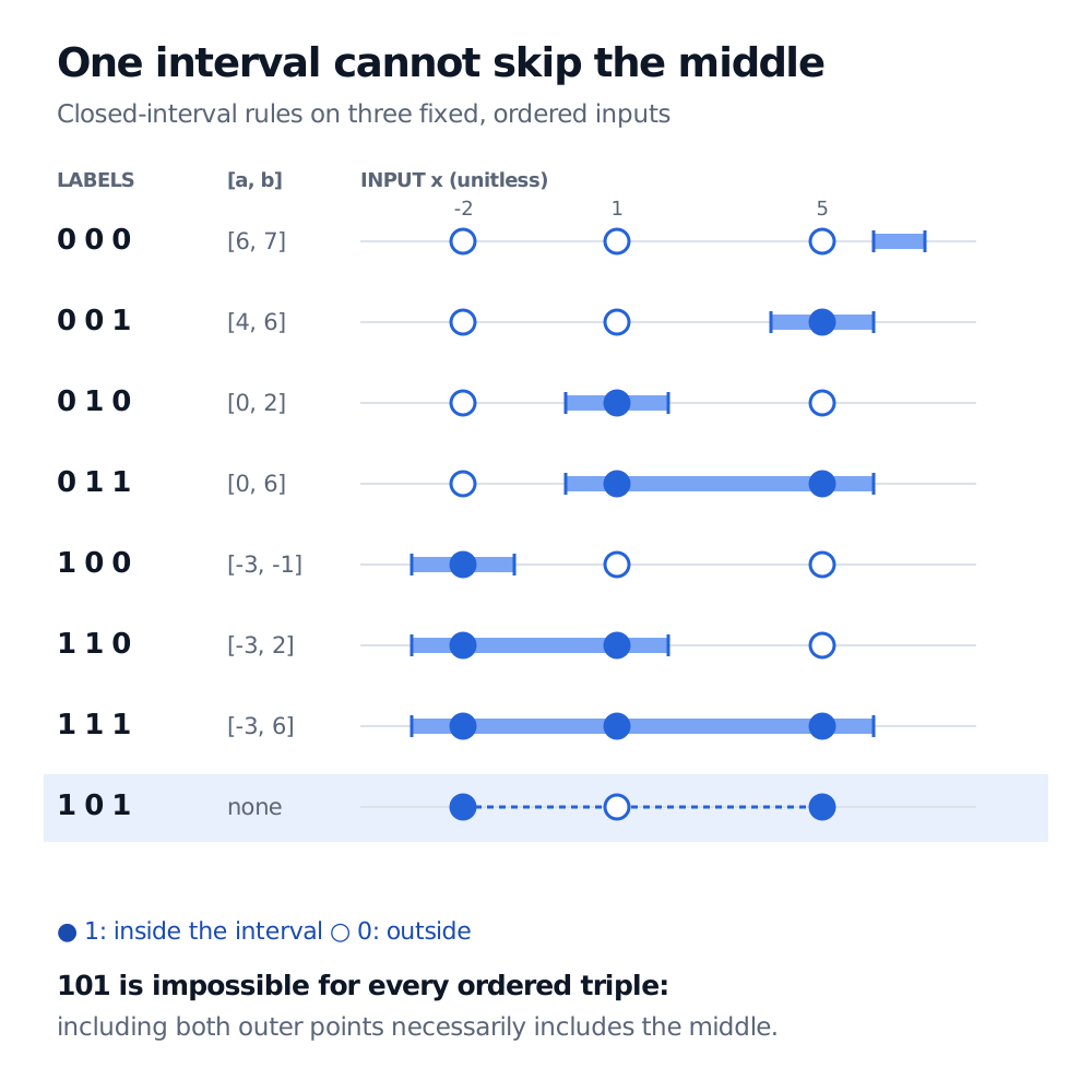
Closed intervals on inputs −2, 1 and 5 realise 000, 001, 010, 011, 100, 110 and 111. The eighth pattern, 101, is impossible: an interval containing −2 and 5 also contains 1.
Original exact combinatorial example. Each row uses a different closed interval on the same three inputs; filled circles mean label 1. The dashed final row is an impossible request, not a classifier.
For the fixed triple −2,1,5, the seven achievable patterns are 000, 001, 010, 011, 100, 110 and 111. Only 101 is missing. Seven out of eight is still not shattering.
Thresholds are a different class
Fix the orientation of a one-sided threshold:
ht(x)=1{x≥t},t∈R.
One input can receive either label by moving t to either side. For every ordered pair u<v, however, label 10 is impossible: if u≥t, then v≥t too. Thus this class has VC dimension one. Allowing both threshold orientations changes the class; the orientation restriction belongs in the definition.
Intervals use two endpoints, but their dimension of two is a result of the proof, not a parameter-counting rule. For example, writing the same endpoints as a=r+s and b=t+q, constrained by r+s≤t+q, uses four real numbers and leaves exactly the same interval class. Its shattering capacity remains two. Capacity belongs to the functions available, not the redundancy of their coordinates.
Count the patterns as the sample grows
The growth functionΠH(m) is the maximum number of distinct label vectors the class produces on a set of m inputs. Shattering means this maximum reaches 2m.
For intervals, the ones must form a single contiguous block in the ordered inputs. For a block beginning at position i, there are m−i+1 choices of its last position. Including the all-zero pattern gives the exact count
ΠHint(m)=1+i=1∑m(m−i+1)=1+2m(m+1).
At three points this is seven; at ten it is 56, compared with 1,024 unrestricted binary labellings. The class contains infinitely many intervals but produces only finitely many patterns on any fixed finite sample.
More generally, the Sauer–Shelah bound states that a binary class with finite VC dimension d satisfies
In the standard distribution-free binary-classification setting with 0–1 loss, finite VC dimension characterises statistical PAC learnability and uniform convergence of empirical risk. This statement assumes IID training observations from one fixed distribution and the usual measurability conditions: losses and the relevant learner and supremum events must have well-defined probabilities. It is not an unrestricted statement about arbitrary function classes or sampling mechanisms.
Realizable PAC learning assumes a zero-error rule exists in the class. Agnostic PAC learning permits noisy labels and targets error within ε of the best error in the class, with probability at least 1−δ over the training sample. For nontrivial finite VC dimension d, the agnostic sample complexity is of order
ε2d+ln(1/δ),
up to universal constants in the standard theorem. This is a rate, not an exact observation count. Realizable bounds have different accuracy dependence. These distinctions are formalised in Understanding Machine Learning, Theorems 6.7–6.8 and Remark 3.1; statistical learnability also does not guarantee an efficient search algorithm.
For financial data, serial dependence, overlapping labels and distribution shifts can invalidate the IID guarantee. Nor does a classification-error guarantee establish profitability after costs. Use VC dimension to understand a specified model class's capacity; use an evaluation design suited to the market claim to assess generalisation.