Probably approximately correct learning separates prediction accuracy from confidence over training samples. Derive a finite-class guarantee and see its limits for quant research.
PAC learning
PAC learning—probably approximately correct learning—is a framework for asking whether training on enough random examples can produce a predictor with a specified error tolerance and a specified confidence of meeting it. For a quant, it makes “enough data to generalise” a claim with explicit assumptions, rather than a conclusion drawn from a good backtest.
The simplest setting is binary classification. A hypothesis class H is the set of candidate prediction rules. Examples (X,Y) come from a fixed, unknown distribution D, and the true error of a rule h is
LD(h)=P(X,Y)∼D(h(X)=Y).
This is an error probability on a fresh observation, rather than the fraction of mistakes in the training data.
Two tolerances, two experiments
Let S contain m independent and identically distributed observations, and let A(S) be the fitted rule. In the realizable setting, some rule in H has true error zero. The PAC requirement is
PS∼Dm(LD(A(S))≤ε)≥1−δ.
Here ε limits the fitted rule's true error, while δ limits the chance that a randomly drawn training sample leads to a rule exceeding that limit. A class is PAC learnable if one algorithm and a finite sample-size function work for every pair ε,δ∈(0,1) and every distribution satisfying realizability. The sample-size function can depend on the class and tolerances, but not on the unknown distribution. MIT's learnability notes explain this distinction.
With ε=0.10 and δ=0.05, at least 95% of possible training samples must produce a rule whose error probability is at most 10%. This does not promise correct predictions at every input, nor a 95% success probability for each prediction. It is also not a posterior probability that a particular already-fitted rule is good.
Why a finite class can be learned
Assume the candidate class is finite and fixed before drawing S, realizability holds, and the learner returns a consistent rule: one making no training mistakes. Exact empirical risk minimisation finds such a rule in this setting because a zero-error rule exists.
Take any fixed bad rule with true error greater than ε. Its probability of escaping detection in all m independent training cases is at most (1−ε)m. A union bound then controls the possibility that any bad rule survives:
PS(LD(A(S))>ε)≤∣H∣(1−ε)m≤∣H∣e−mε.
Consequently, it is sufficient to take
m≥εln(∣H∣/δ).
This is the consistent finite-class theorem proved in Cornell's PAC lecture, Theorem 2.1. The bound covers selection among the entire class, so the final rule may depend on the training sample. The union bound does not require the candidate rules' failure events to be independent.
For a fixed class of 100 rules and the tolerances above,
m≥0.10ln(100/0.05)=76.0090…,m=77 suffices.
At that sample size, the two bounds are
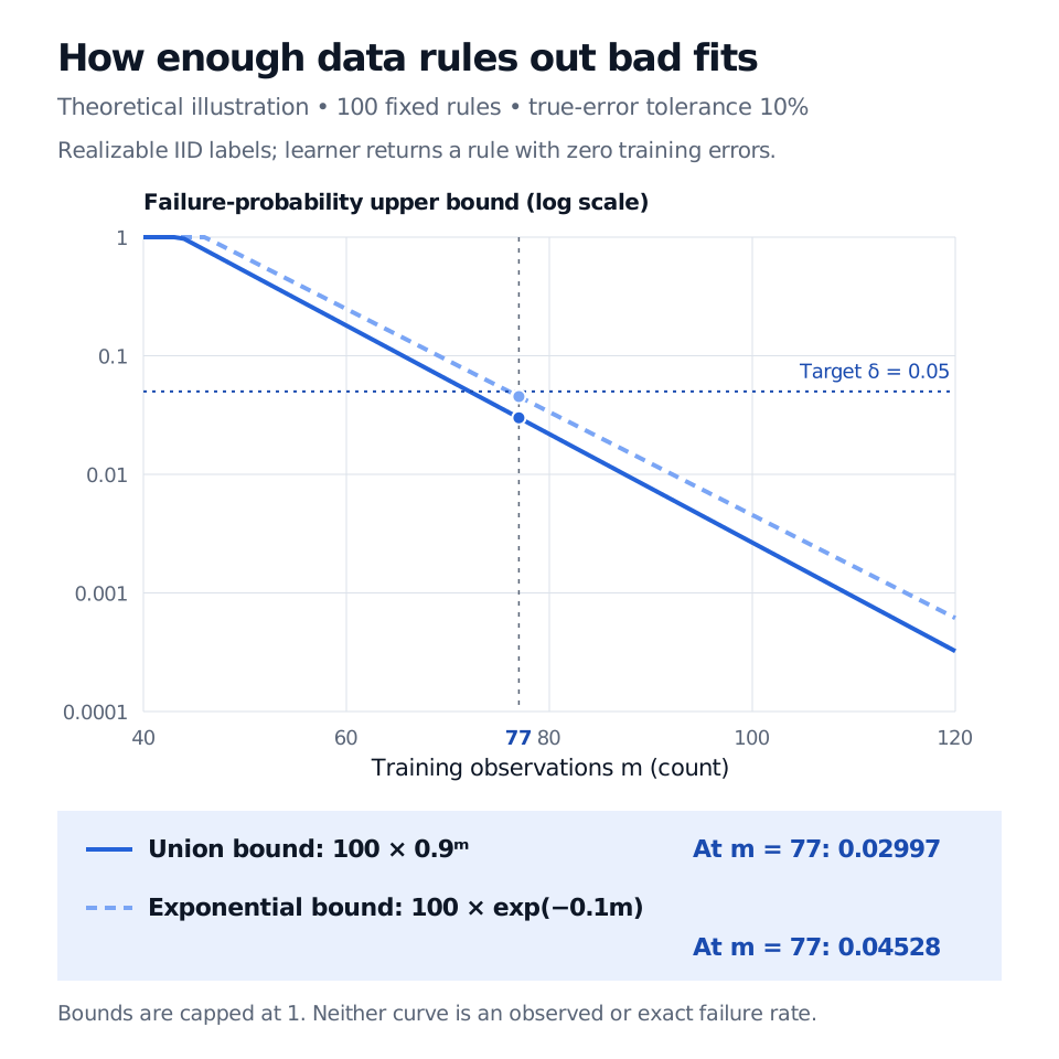
100(0.9)77≈0.0299691,100e−7.7≈0.0452827<0.05.
Neither number is the actual probability of failure. Both are upper bounds, and 77 is a sufficient size from this particular exponential argument, not a universal minimum.
For a fixed class of 100 rules, realizable IID binary labels and zero training error, 77 observations give a union upper bound of 0.02997 and an exponential upper bound of 0.04528 on failure to attain true error at most 10%. Both bounds are below 0.05; neither curve is an exact failure rate.
Original theoretical illustration, with a logarithmic probability axis and bounds capped at one. The 77-observation threshold comes from the looser exponential bound; the sharper union bound can certify the target earlier. This is not a market-data experiment.
When zero population error is unavailable
Noisy labels or a restricted model family can make realizability false. Agnostic PAC learning instead aims to get close to the best rule in the chosen class:
PS(LD(A(S))≤h∈HinfLD(h)+ε)≥1−δ.
The error allowance is now excess error within the class. Even perfect learning by this definition may leave substantial absolute error. For a finite class with 0–1 loss, a standard uniform-convergence argument gives sufficient sample size of order (ln∣H∣+ln(1/δ))/ε2, rather than the realizable argument's 1/ε dependence.
Infinite classes can also be learnable. In the standard measurable IID binary-classification setting with 0–1 loss, the fundamental theorem connects finite VC dimension, uniform convergence of empirical risk, realizable PAC learnability and agnostic PAC learnability. This equivalence concerns statistical learnability; it does not give the same sample bound in the two settings. See Understanding Machine Learning, Definition 3.3 and Theorem 6.7.
A separate question is whether the learner can find its rule efficiently. A sample bound counts observations; a computational bound counts work. Searching a huge class can be prohibitively slow even when its logarithm gives a manageable sample bound. Columbia's lecture separates these questions.
What this means for a quant's model search
The class size must account for the search actually available to the learner. Picking 100 finalists after an unrestricted feature and strategy search does not justify applying the 100-rule theorem to the data that drove that search. Fix the class before the training sample for this argument, or use a result that accounts for the larger, adaptive procedure. Keep the final test set separate from class design and selection.
Financial observations can share overlapping labels, depend across time and come from changing market conditions. Those features break the IID, common-distribution assumptions of this calculation; 77 historical rows do not automatically carry its guarantee. Furthermore, a classification error limit alone says nothing about payoff sizes, turnover or transaction costs. PAC theory clarifies what would establish generalisation under a specified model of sampling; the sampling model must fit the claim.
For the next mathematical step, Sample Complexity Bounds: Finite and Infinite Hypothesis Classes develops the finite-class uniform bound and the two-error-term argument for empirical risk minimisation. The full lesson requires membership; a public preview is available.
Sources
MIT 6.790, Learnability and VC Dimension, especially Realizability, the accuracy/confidence parameters and PAC Learnability.