QuantGAN uses temporal adversarial networks to simulate financial returns. An eight-position receptive-field example separates architecture from validated tail risk, pricing and trading performance.
QuantGAN
QuantGAN is a family of generative adversarial models that uses temporal convolutional networks to simulate financial return sequences. Its practical attraction is a learned path simulator: synthetic observations can reproduce patterns across time, rather than merely matching a one-day return histogram. Wiese, Knobloch, Korn and Kretschmer introduced the method in Quant GANs: Deep Generation of Financial Time Series. Original paper, Introduction
The adversarial part and the temporal part
A generative adversarial network trains two opponents. A generator transforms random noise into samples; a discriminator learns to distinguish generated samples from training observations. The generator learns through that comparison. After training, sampling uses the generator, without needing the discriminator to approve each path. Goodfellow et al., abstract
A temporal convolutional network applies filters across sequence positions. Causal filters use the current and earlier positions; dilation spaces their taps apart to enlarge the receptive field. This is an architectural information constraint, not a claim of economic causation. Bai, Kolter and Koltun, §§3.1–3.3
The QuantGAN paper studies both a direct TCN return generator and a stochastic-volatility neural network that separates drift, volatility and innovations. Temporal dependence supports features such as volatility clustering. Wiese et al., §§5.1 and 7.2
Eight positions, not eight days of forecasting skill
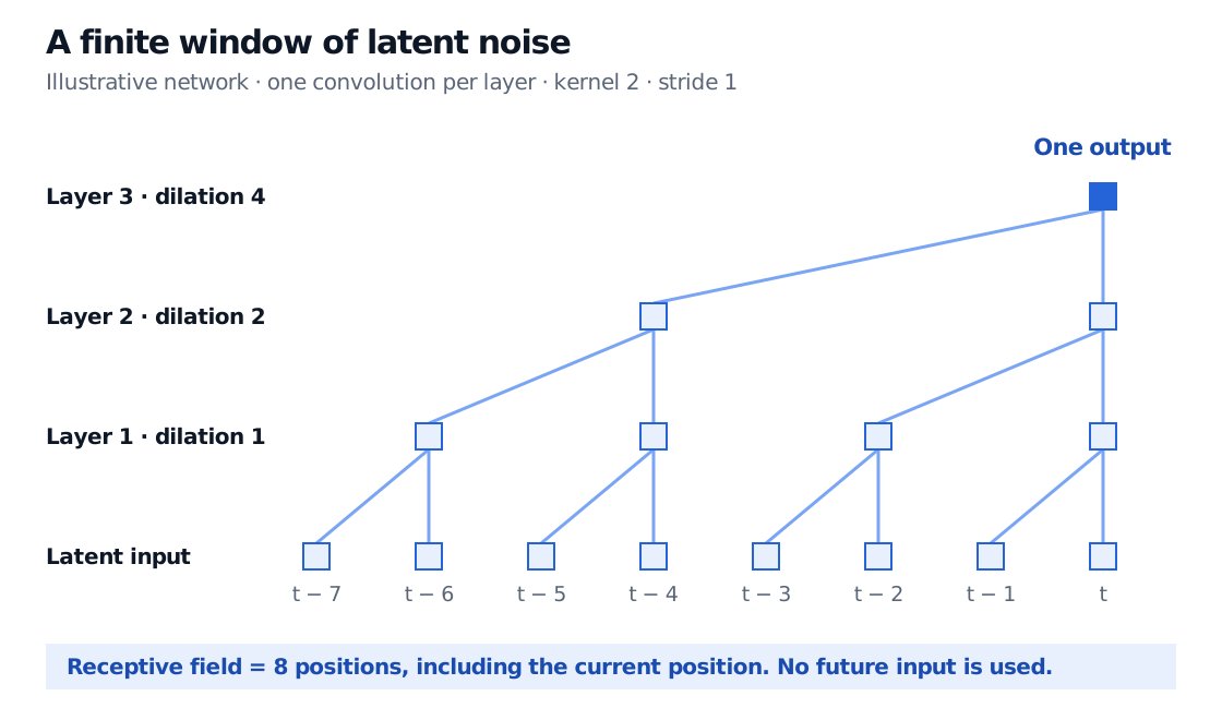
Consider an illustrative causal network with three layers, exactly one convolution per layer, kernel size k=2, stride one and dilations d1=1, d2=2, d3=4. Pointwise activations do not expand its temporal support. Away from the left boundary, its receptive-field span is
R=1+ℓ=1∑3(k−1)dℓ=1+(2−1)(1+2+4)=8.
The initial one counts the current position. Trace the two choices at each filter backwards: the possible input offsets are every integer from zero through seven. Thus an output at time t can depend on inputs from t−7 through t, inclusive. It cannot use t+1.
An illustrative causal network has one kernel-size-two convolution per layer with dilations 1, 2 and 4. One final output at t receives information from eight latent-input positions, t minus 7 through t, with no future input.
Three single-convolution layers cover eight latent positions. This is a connectivity illustration, not a fitted model or a financial performance result.
The figure traces potential connections. Learned zero weights or inactive units can reduce actual sensitivity, so “can depend” does not mean that every input materially affects every generated return. Nor does a window of latent noise mean that the simulator conditions on eight observed market returns. Generating a plausible sequence and forecasting tomorrow from today's observed information are different tasks.
This is not the paper's literal architecture. Its Appendix B uses two convolutions per temporal block and reports a receptive field of 127 positions. Count convolutions, kernel sizes, dilations and strides before quoting a receptive field. Wiese et al., Appendix B
A realistic path still needs a task-specific test
The original study compares generated and historical return distributions and dependence statistics. Its conclusion leaves exact tail modelling and extrapolation as open challenges. Wiese et al., §§7–8
That distinction matters when deciding what a simulator can support:
Intended use
Evidence still needed
Synthetic research scenarios
Diversity, dependence and behaviour across untouched market periods; check whether stressed regimes are represented.
Tail-risk estimation
Tail-sensitive validation at the loss horizon of interest, with uncertainty around scarce extreme observations. A close central histogram does not validate expected shortfall.
Derivative valuation
A specified pricing measure and calibration to relevant instruments, together with the required no-arbitrage restrictions.
Strategy assessment
Evaluation on untouched real data, with trading costs, decision timing and executable prices. Profits on generated paths alone cannot establish a tradable edge.
These are implications for using a learned simulator, not additional empirical results claimed by the paper. Generating more paths reduces simulation noise under the fitted model; it does not supply new independent evidence that the fitted model describes an unseen crisis.
The paper also develops a martingale correction for its structured generator. That construction is distinct from fitting historical returns, and option-price calibration is left as future work. A successful historical fit alone therefore does not establish a calibrated risk-neutral measure or an arbitrage-free pricing system for a collection of traded derivatives. Wiese et al., §5.4