Evaluate an uplift ranking with treated-versus-control response counts, an explicit scaling convention and a random-ranking baseline.
Qini curve and uplift evaluation
A Qini curve evaluates an uplift model's ranking by plotting estimated incremental outcomes as progressively more of the highest-scored population is selected. For a quant team testing a customer-retention intervention, it asks whether limited treatment capacity is directed towards groups whose response changes most, rather than simply towards customers likely to respond anyway.
The score typically estimates a conditional average treatment effect. Evaluation compares treated and control groups within score ranges; it never reveals which particular person's response was caused by treatment.
Fix the counting convention first
Rank a held-out trial population by decreasing predicted uplift, using pretreatment features. At a prefix containing the top k people across both arms, let Nt(k),Nc(k) be the treated and control counts, and Yt(k),Yc(k) their numbers of positive binary responses. This article uses the prefix-scaled count convention
The ordinate is an estimated incremental response count at the prefix's treated-group size, not a response rate or the gain from treating all k people. Belbahri et al., §2.3 give this count construction before discussing normalized versions.
Use prefixes with both arms represented; the displayed rate comparison is undefined otherwise. Group tied scores together or fix an outcome-independent tie rule. Recompute the cumulative comparison at each prefix: adding separately scaled bin gains need not give the same result.
Forty people, four incremental responses
Consider a fictional held-out trial of 100 people with equal-probability randomized assignment. These are stipulated cumulative counts, not fitted model results.
Ranked prefix
Treated people
Treated responses
Control people
Control responses
Q(k)
Top 40
20
8
20
4
4
All 100
50
15
50
10
5
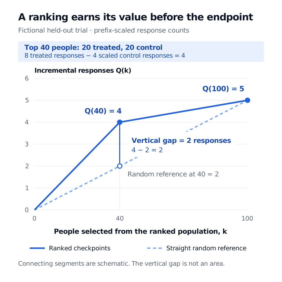
At the top 40, response rates are 40% and 20%. The difference is 20 percentage points, and scaling it to the 20 treated people gives Q(40)=4. Across all 100, the rates are 30% and 20%, giving Q(100)=5. Neither calculation identifies four or five individually caused responses.
Define the straight random-ranking reference as R(k)=(k/100)Q(100). At 40 people it is R(40)=2, so the model's vertical excess is 4−2=2 responses. Random ranking is distinct from randomized treatment assignment. This line is a comparison convention, not a guarantee that every finite random prefix yields exactly that value.
Fictional held-out trial: the top 40 of 100 people have count-scaled Qini 4 versus random-ranking reference 2; at all 100 people both meet at 5. The vertical gap at 40 is 2 responses, not an area.
Original fictional example using prefix-specific treatment/control scaling. Lines between the stipulated checkpoints are schematic; the full empirical curve is not supplied.
Every ranking of these same observations reaches the same full-sample endpoint. The useful distinction is where the incremental gain accumulates before that endpoint.
Ranking quality is not effect calibration
A common Qini summary is the area between the model curve and the straight reference, integrated over selection depth. The two-response gap at 40 is one height, not that area. Raw areas, areas above baseline and normalized coefficients are different quantities; report the formula, axes, scaling and tie handling before comparing scores labelled “Qini” or “AUUC.” Some implementations use a whole-sample arm ratio rather than the prefix ratio used here.
A strictly increasing transformation of scores preserves the ranking and its curve, even if the numerical effect predictions become badly calibrated. Radcliffe and Surry, §§4.1–4.3 distinguish ranking, calibration and impact at a chosen cutoff. Curves can cross: an overall area winner need not win at the actual treatment capacity. Response gain also excludes treatment cost and response value; a profitable allocation needs those quantities too.
What makes the comparison causal
The simple count comparison suits a trial with a common randomized assignment probability, consistent treatment definitions, no interference between people and comparable outcome observation over a fixed horizon. Tiny prefixes remain noisy even with randomization; a rising line alone supplies no uncertainty assessment.
In observational data, multiplying control counts by an arm-size ratio does not remove confounding. Causal evaluation needs conditional exchangeability, consistency and overlap, together with an appropriate adjustment such as propensity weighting or doubly robust estimation. The multi-armed Qini paper, §3, separates model training from test-sample policy evaluation and states overlap and unconfoundedness explicitly.
Keep evaluation outcomes out of ranking-model training and tuning. Selecting the model or cutoff by repeatedly inspecting a test curve uses that test set for selection; reserve fresh evaluation data. For financial applications, the split must also respect the decision's information cutoff and dependencies. Interpret the resulting curve as evidence about group targeting under the study design, not verified individual causal responses.