Probabilistic and sparse PCA: Definition & Examples

Probabilistic PCA (PPCA) gives principal component analysis a Gaussian latent-variable model with equal residual variance in every feature direction. Sparse PCA changes the fitting problem to favour component loadings with exact zeros. For a quant compressing a panel of market measurements, the distinction is practical: PPCA supplies a probability model and uncertainty about hidden coordinates; sparsity makes a component depend on fewer recorded features. They are two extensions, and either can be used without the other.

Ordinary PCA performs linear dimensionality reduction. For centred observations with covariance matrix

S

, its first unit loading vector maximises

\mathbf{v}^{T}S\mathbf{v}

. Subsequent orthogonal directions capture the largest remaining variances. A loading says how a feature enters a component; a score is the resulting coordinate for one observation.

PPCA separates latent signal from isotropic noise

Let $\mathbf{x}\in\mathbb{R}^{p}$ be an observation and $\mathbf{z}\in\mathbb{R}^{q}$ a hidden coordinate, with $q<p$ . The model is

\mathbf{x}=\boldsymbol{\mu}+W\mathbf{z}+\boldsymbol{\epsilon},\qquad \mathbf{z}\sim\mathcal{N}(\mathbf{0},I_q),\qquad \boldsymbol{\epsilon}\sim\mathcal{N}(\mathbf{0},\sigma^2I_p),

with independent latent coordinates and noise. Integrating out $\mathbf{z}$ gives

\mathbf{x}\sim\mathcal{N}(\boldsymbol{\mu},C),\qquad C=WW^T+\sigma^2I_p.

“Isotropic” means the same noise variance in every direction. General factor analysis instead allows a diagonal residual covariance with different feature-specific variances. This distinction is about the noise model, not sparse loadings. See the maintainers’ comparison of factor analysis and PPCA.

For complete data, use covariance $S$ calculated with divisor $n$ and descending eigenvalues $\lambda_1,\ldots,\lambda_p$ . At a nondegenerate maximum-likelihood solution,

\widehat{\sigma}^2=\frac{1}{p-q}\sum_{j=q+1}^{p}\lambda_j, \qquad \widehat{W}=U_q(\Lambda_q-\widehat{\sigma}^2I_q)^{1/2}R.

Here

U_q

contains the leading eigenvectors,

\Lambda_q

their eigenvalues and

R

is orthogonal. Thus PPCA recovers the principal subspace, while latent orientation remains ambiguous. Its loading matrix is not generally the unit PCA loading matrix. These results and the posterior below are derived in Tipping and Bishop (1999), Section 3.

A hidden coordinate is not a raw PCA score

Take two centred, dimensionless features with stipulated population covariance

C=\begin{pmatrix}4&0\\0&1\end{pmatrix},\qquad q=1.

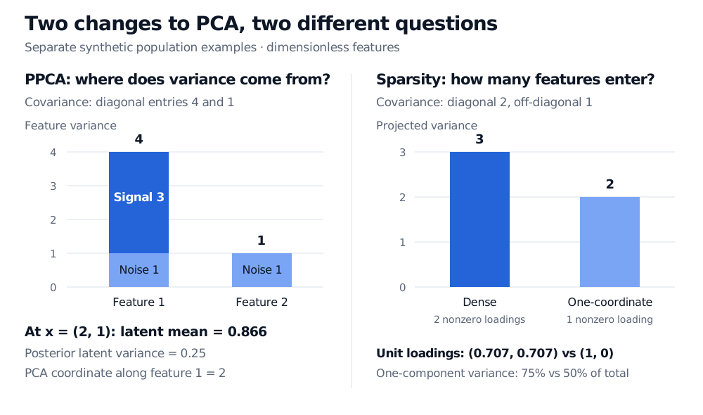
One exact PPCA representation is $\sigma^2=1$ and $W=(\sqrt{3},0)^T$ . Feature 1 has signal variance $3$ plus noise variance $1$ ; feature 2 has only noise variance $1$ . These are model assumptions for a synthetic example, not estimated market quantities.

For an observed $\mathbf{x}=(2,1)^T$ , set $M=W^TW+\sigma^2I_q$ . Gaussian conditioning gives

\mathbb{E}[\mathbf{z}\mid\mathbf{x}] =M^{-1}W^T(\mathbf{x}-\boldsymbol{\mu}) =\frac{\sqrt{3}}{4}\,2 =\frac{\sqrt{3}}{2}\approx0.866,

and posterior latent variance $\sigma^2M^{-1}=1/4$ . The ordinary PCA score along $(1,0)^T$ is $2$ . The two coordinates use different scales, and PPCA inference also incorporates noise. Multiplying the posterior mean by $W$ gives the conditional mean of the latent signal, $(1.5,0)^T$ ; the ordinary orthogonal projection is $(2,0)^T$ . Neither numerical difference indicates that a PCA direction was misidentified.

Two separate synthetic examples: PPCA decomposes feature variances 4 and 1 into signal variances 3 and 0 plus noise variance 1 each; its latent posterior mean at (2,1) is 0.866 with variance 0.25. For covariance with diagonal 2 and off-diagonal 1, a dense unit loading captures variance 3, versus 2 for a one-coordinate unit loading.

Original population examples with dimensionless features. Left: equal noise variance does not imply equal total variance. Right: limiting a component to one feature sacrifices projected variance in this example; it does not illustrate a fitted penalty path.

Sparse PCA changes what a component may use

Sparse PCA seeks loadings with fewer nonzero entries. A particular method must specify its objective, constraints and normalisation. For example, Zou, Hastie and Tibshirani (2006), Section 3.2 use the regression-type criterion

\min_{A,B}\; \lVert X-XBA^T\rVert_F^2 +\lambda\sum_{j=1}^{q}\lVert\boldsymbol{\beta}_j\rVert_2^2 +\sum_{j=1}^{q}\lambda_{1,j}\lVert\boldsymbol{\beta}_j\rVert_1, \qquad A^TA=I_q.

X

has centred observations in rows;

A

and

B

are

p\times q

, and

\boldsymbol{\beta}_j

is column

j

B

. The L1 penalty encourages zeros; nonzero fitted columns of

B

are normalised to give sparse loadings. Orthogonality of

A

does not imply orthogonal sparse loadings or uncorrelated component scores. The authors discuss the resulting variance-accounting problem in Section 3.4: simply adding correlated score variances can overstate distinct information captured.

A small calculation isolates the cost of restricting support. For a different population covariance,

S=\begin{pmatrix}2&1\\1&2\end{pmatrix},

the dense leading unit loading $(1,1)^T/\sqrt{2}$ captures variance $3$ . If a unit loading must have exactly one nonzero entry, it must choose one coordinate, capturing variance $2$ . Relative to total variance $4$ , those single-component shares are $75\%$ and $50\%$ . This is an explicit support constraint, not the output of an unspecified sparse PCA implementation. Either coordinate is equally good here: sparsity does not ensure a unique selected feature.

Other methods solve different problems. For instance, scikit-learn’s SparsePCA uses a dictionary-learning reconstruction objective with an L1 penalty, rather than the criterion displayed above. A package name alone does not determine how scores, reconstruction and explained variance should be compared.

For market data, choose feature units and scaling deliberately: rescaling changes both the variance geometry and the effective cost of penalising coefficients. A sparse loading is an interpretable measurement recipe, not evidence that excluded variables have no economic role. A Gaussian PPCA fit likewise does not establish Gaussian tails or equal residual noise in observed returns.

For the underlying projection geometry, Principal Component Analysis and the SVD View derives the maximum-variance direction and reconstruction interpretation. The preview is public; the full lesson requires membership.

Sources

Tipping and Bishop (1999), Mixtures of Probabilistic Principal Component Analysers, Sections 2.2–3.3: the single PPCA model, maximum-likelihood solution and posterior coordinates.
Zou, Hastie and Tibshirani (2006), Sparse Principal Component Analysis, Sections 3.2–3.4: penalised regression formulation, normalisation and adjusted variance.
Scikit-learn, Decomposing signals in components, Sections 2.5.1.1, 2.5.1.4 and 2.5.5: current implementation distinctions and residual covariance assumptions.

PPCA separates latent signal from isotropic noise

A hidden coordinate is not a raw PCA score

Sparse PCA changes what a component may use

Sources

Related terms

Dimensionality reduction

Eigenvector

Factor analysis

L1 regularization