Pre-FOMC announcement drift is the historically observed tendency for U.S. equities to earn unusually high average returns in the hours before scheduled monetary policy announcements by the Federal Open Market Committee (FOMC). In an event study, it matters whether prices moved before the statement was public or in response to the news it contained. A single close-to-close return can blend those two moves. Lucca and Moench, New York Fed Staff Report 512.
Which timestamp ends the window?
In Lucca and Moench's September 1994–March 2011 sample of 131 scheduled announcements, the S&P 500 earned an average excess return of about 49 basis points from 2:00 p.m. Eastern Time on the previous day to 2:00 p.m. on announcement day. Statements usually came out around 2:15 p.m. in that sample. The New York Fed first issued the staff report in 2011, revised it in 2013, and the journal article appeared in 2015. Staff report, Sections 1–3 and Table 2, publication history.
An event window defined by that historical clock needs rechecking when release times change. In 2011 and 2012, some scheduled statements came out at 12:30 p.m. In March 2013, the Fed moved regular statements to 2:00 p.m. Eastern and set news conferences to start around 2:30 p.m. A window ending at 2:00 p.m. could therefore include the statement response in one era and end before it in another. Lucca and Moench's timing update, Federal Reserve timing announcement.
For historical measurement, align prices to the verified public release timestamp. Keep the policy statement and the Chair's press conference as separate events, and flag unscheduled decisions separately. For a calendar-based backtest, use the schedule that was available when the window was set. Moving a historical entry or exit to fit a release time learned later introduces look-ahead bias. The Fed calendar indexes statements and press conferences, while a statement's “for release” header gives its listed time. Intraday data need an explicit price cutoff if a bar at that time could contain trades on both sides of the release. FOMC calendars.
Three meetings, two averages
Take three fictional meetings. Set minute zero to the actual statement release. Measure raw index log returns from minute −60 to −1 in the pre-release window, and from minute +1 to +16 in the post-release window. The immediate jump across the statement falls in the gap. Weight each meeting equally within each window.
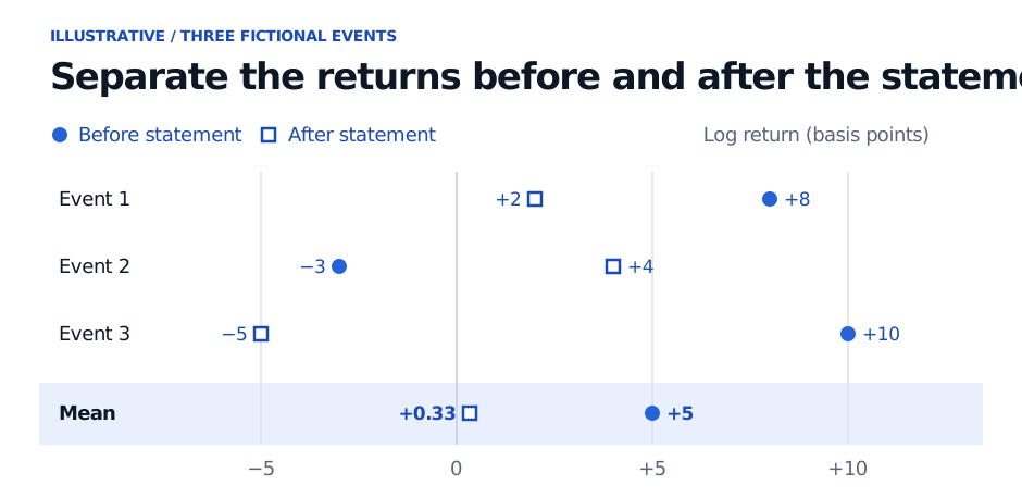
The three fictional meetings produce different averages depending on which side of the statement is measured. The post-release average rounds to +0.33 bp.
The windows have different lengths and measure different periods. A study of whether pre-FOMC returns were unusual would compare the pre-release observations with non-meeting windows of the same length and time of day. It would also state whether it uses raw returns or excess returns over cash, as Lucca and Moench did. A study of the immediate response to a monetary-policy shock would instead use a narrow window spanning the statement and a measure of how policy differed from expectations. Lucca and Moench, Section 3, Knox and Vissing-Jorgensen, Section 2.1.
The SelfMadeQuant lesson works through how to separate a release window from the earlier interval used to estimate a normal return. The event-time excerpt is public, and the full lesson requires membership. Estimation and Event Windows
What happened in later samples?
In a 2018 update using April 2011–June 2018 data, Lucca and Moench found that the pre-statement rise was concentrated in meetings with press conferences. Kurov, Wolfe and Gilbert extended the sample through December 2019 using E-mini S&P 500 futures and found that the drift ahead of press-conference meetings weakened from January 2016. These studies group meetings and set their windows differently. Lucca and Moench, 2018 update, Kurov, Wolfe and Gilbert, Section 2 and Table 2.
In a 2026 Fed working paper, Knox and Vissing-Jorgensen estimated a 16 bp S&P 500 return differential for their fixed 2:00 p.m.–2:00 p.m. window over April 2011–December 2023, statistically indistinguishable from zero at conventional levels. The historical estimates depend on the sample, instrument and clock. They leave the present expected return and profitability after execution costs unmeasured. Knox and Vissing-Jorgensen, Section 5.2 and Table 4.