Poisson regression models a nonnegative integer count using a Poisson distribution whose conditional mean depends on predictors. A quant might use it to estimate how operational-incident frequency changes with a desk's activity, while allowing desks observed for longer to accumulate more incidents. It models event frequency; monetary losses per incident require a separate severity model.
The usual specification is a generalised linear model with a log link. For count , predictors and known exposure ,
The inverse link makes the expected count positive. The log is the canonical link, though Poisson models can use other links with suitable mean constraints. CMU's GLM notes, §§2.2 and 2.4, derive this connection.
A rate of three does not mean three observations
Consider a specified fictional incident model, with exposure measured in operating hours and one dimensionless predictor :
At , the expected rate is 2 incidents per hour. At , it is incidents per hour. A two-hour observation therefore has
The predictor and exposure do different jobs:
| Change | Held fixed | Consequence |
|---|---|---|
| Increase from 0 to 1 | Exposure and other predictors | Rate multiplied by |
| Increase exposure from 1 to 2 hours | Predictors and hourly rate | Expected count doubled |
The term is an offset with coefficient fixed at one. Estimating its coefficient instead would allow a different exposure scaling. Proportional scaling assumes the modelled rate remains applicable over the observation's exposure. statsmodels documents both exposure and offset conventions.
Units matter. Three incidents per hour is per minute; using minutes still gives mean . A half-hour at the same predictors gives mean . Expected counts need not be integers; realised counts must be . Fitting the raw counts with their exposure preserves that distinction. A noninteger count-per-hour response is not itself a Poisson count.
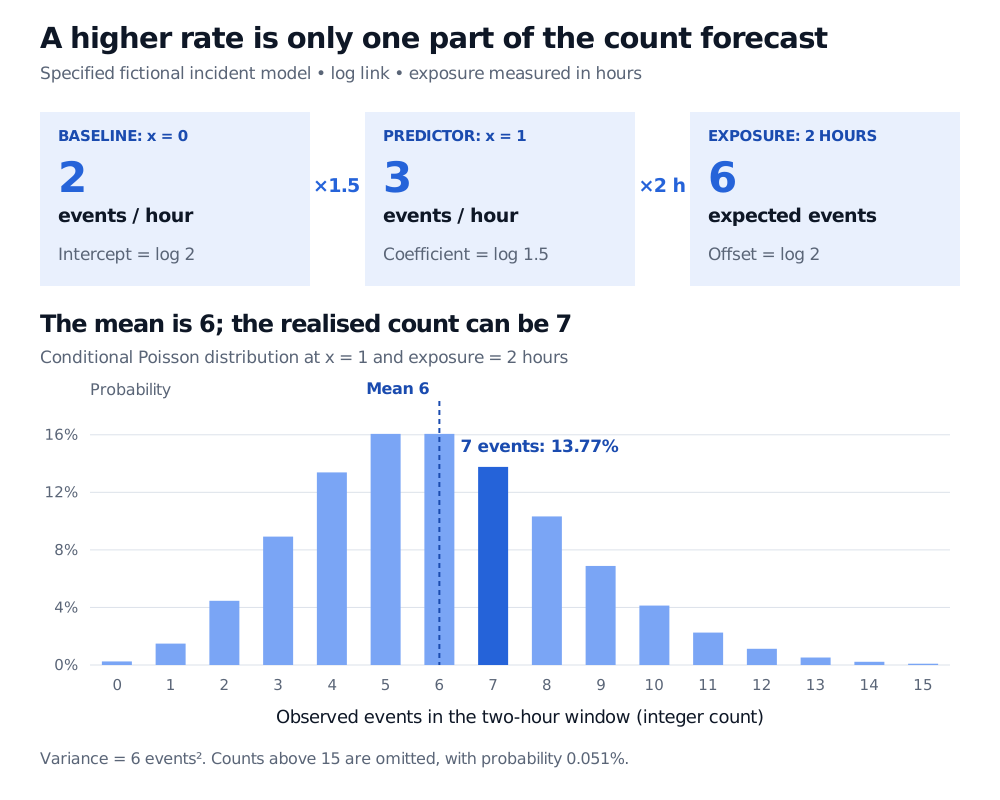
Original specified model, not fitted observations. The upper panel separates a covariate rate multiplier from exposure; the lower panel shows that the resulting expected count is not a guaranteed outcome.
Under the conditional Poisson law, mean also implies variance in squared incident-count units. Seven incidents remain possible:
The model assigns seven incidents a 13.77% probability. The expected count describes an average, while the probability distribution describes variation around it. R's Poisson documentation gives the count support, mass function and moments.
Interpret coefficients on the right scale
For a one-unit change in a predictor appearing as an additive linear term, is the conditional rate ratio, holding other predictors fixed. At fixed exposure, it is also the expected-count ratio. Here means a 50% higher rate, not an extra incidents or a 50-percentage-point probability increase. Interactions require evaluating the full predictor change. These are regression associations; the coefficient alone does not identify a causal effect.
For conditionally independent observations, maximum likelihood estimation fits the coefficients by maximising
with an intercept included in the coefficient vector here. The log link transforms the conditional mean, not the observed count. Ordinary least squares on targets a different quantity and cannot directly accommodate zeros. CMU's estimation section explains likelihood fitting for GLMs.
The owned lesson The Exponential Family and Generalized Linear Models includes a fitted Poisson trade-count example. Its public preview is open; the full lesson requires membership.
Equal mean and variance is a conditional assumption
Poisson regression imposes
It does not require the pooled sample variance to match the pooled sample mean. If half a population has conditional Poisson mean and half has mean , the pooled mean is and variance is . By the law of total variance, the pooled variance contains both average within-group variance and variation between group means: . Raw heterogeneity can therefore look overdispersed even when each conditional model is Poisson.
Check residual variation after accounting for predictors and exposure. If substantial extra variation remains, negative binomial regression provides an alternative count distribution; quasi-Poisson relaxes the variance to without specifying a full count likelihood. It is not enough to change a variance assumption if the mean, exposure or dependence structure is wrong. Zeileis, Kleiber and Jackman, §2.1, compare these approaches; R's family documentation explains the unfixed quasi-Poisson dispersion.
Many zeros are also not a diagnosis. Compare them with probabilities from an appropriate fitted model, including varying means and exposure. A zero-inflated distribution adds a separate point-mass component at zero; a hurdle model separates zero from positive outcomes. Both introduce mechanisms beyond ordinary Poisson variation. Overdispersion or excess zeros alone does not establish which mechanism generated the data. The count-model paper, §§2.2–2.3, sets out that distinction.