See how decisions made from a forecast shift its target distribution, and why the forecast that retraining settles on can differ from the one with lowest deployment loss.
Performative prediction and model feedback loops
Performative prediction occurs when acting on a model's predictions changes the distribution of the data the model aims to predict. A credit score can affect the interest rate offered, which in turn can affect repayment. Perdomo and colleagues use this stylised example to show how a model can help produce the defaults it is later judged against. A validation set collected under the old lending policy measures performance under that policy. A new policy may produce different outcomes even for comparable borrowers. Perdomo et al., §1
Deployment feedback can resemble exogenous drift in monitoring data. The difference is what causes the shift. A rise in unemployment can change repayment outcomes with the model and loan terms held fixed. Changing the offered terms in response to a score can itself change repayment outcomes. Both can occur at once. A comparison before and after a model update combines those effects unless the comparison can isolate the effect of deployment. Perdomo et al., §1.2
What retraining holds fixed
Write D(θ) for the distribution of observations Z produced when model θ is deployed through a specified decision rule, and ℓ(Z,a) for the loss of candidate model a on one observation. When retraining on data from the incumbent θt, the population update uses one distribution for every candidate.
θt+1∈argaminEZ∼D(θt)[ℓ(Z,a)].
A model is performatively stable if it minimises expected loss on the distribution it already induces. It is a fixed point of exact population retraining when the minimiser is unique. Performative optimality compares candidates by deploying each one and scoring it on its own resulting data.
R(a)=EZ∼D(a)[ℓ(Z,a)].
Minimising R(a) changes both the model and the distribution against which it is scored. Retraining only changes the model used to score the incumbent distribution. Perdomo et al., §§2–3
A forecast that moves its own target
Suppose a fictional desk uses a constant forecast θ of the next-window midpoint change, in basis points. Its trading rule trades against the forecast, with order size proportional to the forecast magnitude. In this toy model, with equal probability, the realised change Y is 3 bps in windows where trading has no price effect and 3−θ bps where it does. The response is stipulated and stays the same across rounds. It represents a mechanism for market impact, with no claim about the shape or magnitude of real price responses.
On data from deployment θ, the best constant under mean squared error is the induced mean, 3−θ/2. If each round uses the exact population mean from the preceding deployment, retraining gives
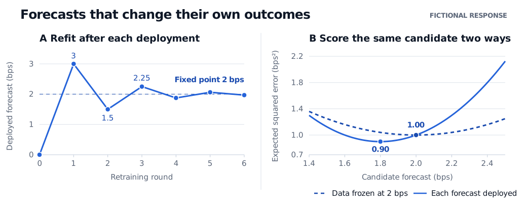
θt+1=3−2θt,0→3→1.5→2.25→⋯.
The fixed point solves θ=3−θ/2, so θ=2 bps. Each update multiplies the signed distance from 2 by −1/2. The forecasts alternate around 2 with half the previous error magnitude. This convergence comes from the stipulated response. A stronger response can make repeated retraining fail to converge. Perdomo et al., §3.2
Now compare deploying a candidate a with merely scoring it on the data from θ=2. Under its own deployment a faces outcomes 3 and 3−a, so
R(a)=21(3−a)2+21(3−2a)2=109+25(a−1.8)2.
The performative optimum is 1.8 bps, with expected squared error 0.90 bps². The stable forecast of 2 bps has expected squared error 1.00 bps². In contrast, scoring 1.8 on the frozen outcomes from θ=2, namely 3 and 1 bps, gives 1.04 bps². The lower forecast looks worse on the incumbent data. Under deployment it reduces the trading response, moving the lower outcome from 1 to 1.2 bps and narrowing the distance between the two possible outcomes. These losses measure forecast error. A desk assessing a trading rule would also need to account for execution costs and P&L.
Fictional example in two panels. Retraining goes from 0 to 3 to 1.5 to 2.25 basis points and approaches 2. The frozen-data error is lowest at 2 basis points with error 1.00 basis points squared. The deployment error is lowest at 1.8 basis points with error 0.90 basis points squared.
The left panel shows the exact population updates. The right panel compares scoring on outcomes generated by the incumbent forecast of 2 bps with scoring each forecast on the outcomes it would generate after deployment.
A desk can record the deployed model version, the orders it prompted and the observed price response. To estimate what a different policy would have produced, it still needs a credible comparison, such as controlled variation in deployment that accounts for concurrent market movements and order interaction. The SelfMadeQuant lesson works through the difference between a move observed after an order and the move attributable to that order. Market Impact (public preview, full lesson for members)