Planning with a probability distribution over hidden states, including a two-state belief update and the distinction between filtering and choosing an action.
Partially observable Markov decision process
A partially observable Markov decision process (POMDP) is a sequential decision model in which actions affect a hidden state and the decision maker receives observations that need not reveal that state. For a quant execution model, the distinction matters when visible quotes and trades provide incomplete evidence about liquidity: an action must account for several possible conditions, rather than treating an estimated regime as known.
Three things that must stay separate
The state is the model’s underlying situation; the observation is the information received; the belief state is a probability distribution over possible states given the available history. A positive signal is an observation. “Good with probability 60%, Bad with probability 40%” is a belief state.
A finite POMDP specifies states, actions, transition probabilities, rewards and an observation model, together with an initial belief and a planning horizon or discount convention. Under its assumptions, the correctly computed belief summarises the history needed for planning. A policy therefore chooses from beliefs, rather than directly from the unobserved state. Kaelbling, Littman and Cassandra (1998), §§3.1–3.4
One observation, with the state held fixed
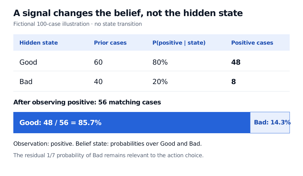
Consider a fictional hidden condition, Good or Bad. Before a signal arrives, the probabilities are 0.6 and 0.4. A positive signal occurs with probability 0.8 in Good and 0.2 in Bad. For this single update there is no state transition.
The posterior probability of Good is about 85.7%; Bad still has probability 1/7, about 14.3%. The observation has not changed Good into Bad or disclosed the true state.
Fictional no-transition example: of 100 prior cases, 60 are Good and 40 Bad. A positive signal selects 48 Good and 8 Bad cases, giving posterior probabilities 85.7% Good and 14.3% Bad.
Original count interpretation of a single Bayesian observation update. The counts illustrate stipulated probabilities; they are not market data or a fitted regime model.
To see why the remaining uncertainty matters, add a terminal decision. Action A earns +2 reward units in Good and −5 in Bad; action B earns zero in either state. Before the signal, A’s expected reward is 0.6(2)+0.4(−5)=−0.8. After the positive signal it is (6/7)2+(1/7)(−5)=1. An expected-reward maximiser chooses B before this signal and A after it. Selecting A still permits a loss of 5 units. These stipulated payoffs illustrate a decision, not a trading rule.
A full step predicts, then corrects
Use the timing “choose action, transition, observe.” Write T(s′∣s,a) for the transition kernel and O(o∣s′,a) for the observation likelihood. From belief bt, action at first gives the predicted distribution
The denominator must be positive. A zero denominator means the observation was impossible under the supplied model. The example above uses an identity transition, so prediction leaves the prior unchanged.
Filtering produces a belief; planning chooses an action using rewards and possible future beliefs. An action may be worthwhile partly because it improves later decisions through information. Replacing the belief with its most likely state can discard that value. Even a finite hidden-state model produces a continuous space of probability distributions, making planning harder. Cassandra, Kaelbling and Littman (1994), “Adding Partial Observability” and “Constructing Optimal Policies”
A POMDP can be specified with known dynamics; it does not inherently require reinforcement learning. Learning those dynamics adds model-estimation uncertainty. In markets, neither the framework nor a concentrated belief guarantees that a latent regime is identifiable, stable or correctly specified. Observations with identical likelihoods across states cannot distinguish those states in the update. Historical evaluation must also reconstruct information available at each decision time.