Orthogonal matching pursuit: Definition & Examples

Orthogonal matching pursuit (OMP) is a greedy method for building a sparse linear approximation: select the dictionary column most strongly aligned with the current residual, then refit all selected coefficients by least squares. A quant researcher can use it to form a compact return model from a larger set of candidate signals or factor histories. The selected columns describe an in-sample fit; selection alone does not establish economic importance or future predictive value.

A dictionary is a matrix of candidate columns, also called atoms. In regression, each atom is one feature's values across the training observations. The word “orthogonal” describes the fitted residual's relationship to the selected span. The dictionary itself need not be orthogonal.

Select one column; reconsider every coefficient

Let $A$ have $n$ rows and $p$ real-valued columns $a_j$ , and let $y\in\mathbb{R}^n$ be the target. Use unit-length columns, $\lVert a_j\rVert_2=1$ . This description fits no intercept; for a regression with an unpenalised intercept, first centre the training features and target, normalise the nonconstant feature columns, and recover the intercept afterwards. Remove zero-length columns.

Start with selected set $S_0=\varnothing$ and residual $r_0=y$ . Each iteration has three decisions:

Select: choose an unselected column with the largest absolute residual inner product,

j_k\in\underset{j\notin S_{k-1}}{\arg\max}\;\lvert a_j^\top r_{k-1}\rvert, \qquad S_k=S_{k-1}\cup\{j_k\}.

Refit: let $A_{S_k}$ contain all selected columns and solve

\hat\beta_{S_k}\in\underset{b}{\arg\min}\;\lVert y-A_{S_k}b\rVert_2^2.

Update: set $r_k=y-A_{S_k}\hat\beta_{S_k}$ , then apply the stopping rule.

These are the core steps of Tropp and Gilbert's OMP algorithm, with the stopping choices discussed below. Here “correlation” means an inner-product score, not automatically a Pearson correlation coefficient. Unit norms prevent a column winning merely because its numerical scale is larger. With centred, equally normalised columns, ranking absolute inner products is equivalent to ranking absolute sample correlations with a nonzero residual. The absolute value allows a negatively aligned column to enter with a negative coefficient.

The refit makes the residual perpendicular to every selected column, in exact arithmetic:

A_{S_k}^{\top}r_k=0.

It is the orthogonal projection condition. Enlarging the selected span cannot increase the training residual norm, because the previous fit remains available. It does not guarantee decreasing validation error.

Two coordinates, then two correlated atoms

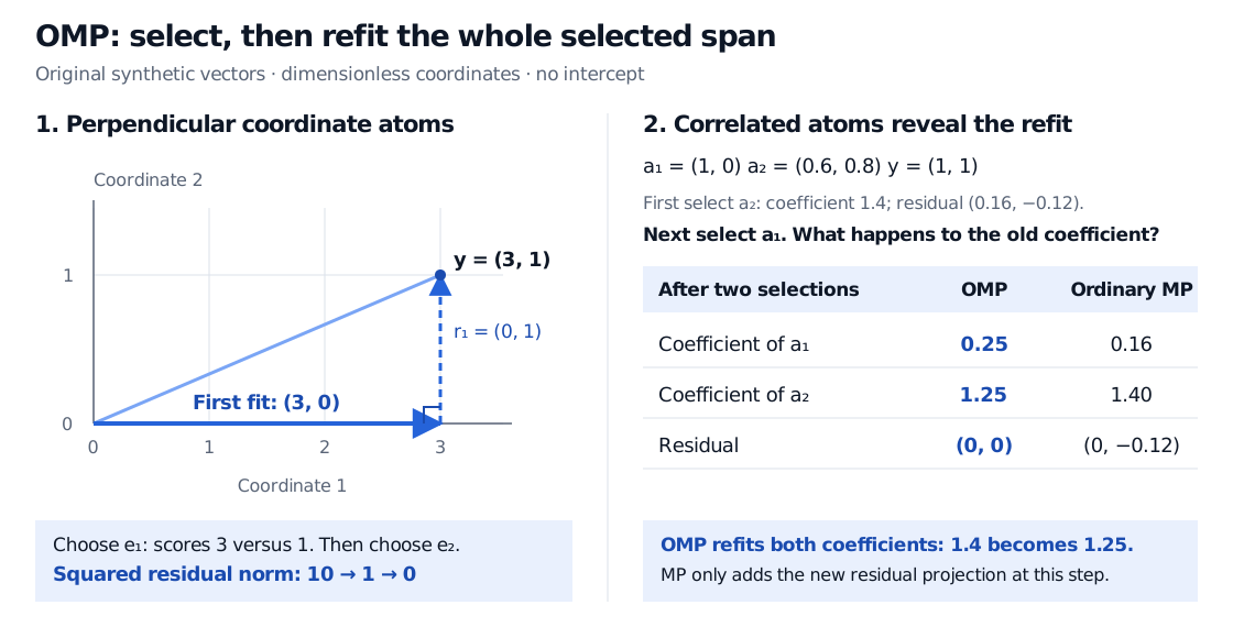
Take the unit coordinate atoms $e_1=(1,0)^\top$ , $e_2=(0,1)^\top$ and target $y=(3,1)^\top$ . This is a dimensionless geometric example without an intercept.

Initially, the absolute scores are 3 and 1. OMP selects $e_1$ , fits its coefficient as 3 and leaves $r_1=(0,1)^\top$ . The residual is perpendicular to $e_1$ . Next it selects $e_2$ and refits on both atoms, giving coefficients $(3,1)^\top$ and zero residual. Squared residual norms fall from 10 to 1 to 0.

Synthetic dimensionless vectors: target (3,1), first fit (3,0), residual (0,1), then exact recovery. With correlated atoms (1,0) and (0.6,0.8) and target (1,1), OMP refits coefficients to 0.25 and 1.25; ordinary matching pursuit after the same two selections keeps 0.16 and 1.4 and leaves residual (0,-0.12).

Original synthetic vectors without an intercept. The left panel shows perpendicular residual geometry; the right compares OMP and ordinary MP after the same two selections. Coordinates and coefficients are dimensionless.

Perpendicular atoms hide the importance of refitting. Instead use unit atoms $a_1=(1,0)^\top$ , $a_2=(0.6,0.8)^\top$ and $y=(1,1)^\top$ . OMP selects $a_2$ first because its score is 1.4, versus 1 for $a_1$ . Its coefficient is 1.4 and the residual is $(0.16,-0.12)^\top$ .

After adding $a_1$ , the joint fit is

0.25a_1+1.25a_2=(1,1)^\top.

The old coefficient changes from 1.4 to 1.25. Ordinary matching pursuit instead adds only the projection of the current residual onto the newly selected atom at this step. It adds

0.16a_1

, retains

1.4a_2

, and leaves residual

(0,-0.12)^\top

. That residual is perpendicular to

a_1

but no longer to

a_2

. Further MP iterations may revisit atoms. This difference is why subtracting one new column's contribution is not an OMP refit.

For the geometry behind the repeated fit, Least Squares and Regression Geometry derives residual orthogonality and the QR solution route. Its preview is public; the full lesson requires membership.

A sparse fit is not a recovery guarantee

OMP is a forward feature-selection procedure. Standard OMP retains selected columns rather than searching all subsets or deleting an earlier choice. Unlike Lasso regression, its refit does not impose an

L^1

penalty on the selected coefficients. It is a greedy approach to a sparsity-constrained problem, not a universal solver for the best subset of a given size. The scikit-learn guide makes that approximation distinction explicit.

Recovery results require assumptions. For example, for unit-norm atoms define coherence

\mu=\max_{i\ne j}\lvert a_i^\top a_j\rvert

. In the noiseless, exactly

s

-sparse setting, the sufficient condition

(2s-1)\mu<1

guarantees OMP recovery of the sparse representation. This is the coherence form of Tropp's recovery bound, not a necessary condition: failing the bound does not prove failure. Noise and approximate sparsity need further analysis. Highly similar financial features also make the selected identity and refitted coefficients sensitive to small data changes, even when fitted values are similar.

Stopping is part of the model

Choose a maximum selected-set size, a residual-error threshold, or a validation-based rule before final evaluation. Stop immediately at zero residual; also handle zero remaining scores, dependent candidate columns and numerical rank failure. Break equal scores deterministically, for example by a fixed column order. Near ties can still make the selected set unstable.

A residual tolerance must specify its convention: a bound on

\lVert r\rVert_2

differs from one on its square. The current scikit-learn OMP API defines tol as a maximum squared residual norm; when supplied, it overrides n_nonzero_coefs. Tolerance therefore also depends on target units and sample size. Exact interpolation of noisy return targets is not a useful default objective.

Fit centring, scaling and OMP selection inside each training split. Tune the selected-set size or stopping threshold using validation within the development data, then assess the frozen procedure on an untouched test. The official leakage guidance applies to both preprocessing and feature selection. For time-indexed return prediction, use time-ordered splits and admit only features and completed training targets available at the fit cutoff. Choosing columns once using all targets before cross-validation leaks held-out information, even if coefficients are subsequently refitted within each fold.

Sources

Tropp, J. A. and Gilbert, A. C. (2007), Signal Recovery from Random Measurements via Orthogonal Matching Pursuit: The Gaussian Case, Caltech Technical Report 2007-01, Algorithm 3, pp. 3–4. Selection, deterministic ties and full least-squares refitting.
Tropp, J. A. (2004), Greed is Good: Algorithmic Results for Sparse Approximation, §§I.C and III.A–C, especially Theorem 3.1 and Corollary 3.6. MP/OMP distinction and sufficient recovery conditions.
scikit-learn developers, Linear Models, §1.1.9: Orthogonal Matching Pursuit, and OrthogonalMatchingPursuit API, parameters n_nonzero_coefs, tol and fit_intercept. Current documentation checked 1 November 2026.
scikit-learn developers, Common pitfalls, §12.2: Data leakage, especially §§12.2.1–12.2.2 on training-only transformations and feature selection.

Select one column; reconsider every coefficient

Two coordinates, then two correlated atoms

A sparse fit is not a recovery guarantee

Stopping is part of the model

Sources

Related terms

Feature selection

Least squares

Orthogonal projection