Oblique trees and model trees: Definition & Examples

An oblique tree routes observations using splits on linear combinations of features. A model tree predicts with a fitted model inside each leaf, commonly a linear regression, rather than a single constant. These are separate choices: one changes where a tree divides feature space; the other changes what it predicts within each region. In quant research, the distinction matters when a joint liquidity–volatility condition defines a regime, but the forecast still varies within that regime.

Two choices, four combinations

A conventional decision tree might split on

x_1>t

. An oblique split can instead use

w_1x_1+w_2x_2>b.

The equality defines a line in two dimensions, or a hyperplane with more features. Several such tests carve out polygonal or polyhedral leaf regions. An axis-aligned tree may need many staircase-like splits to approximate a diagonal boundary. This geometry motivates the original OC1 paper, whose algorithm searches for useful hyperplanes using local coefficient adjustments and randomisation. A smaller tree can still contain more complicated individual tests.

Leaf predictions are a different design decision:

Split tests	Constant numerical leaves	Linear model leaves
One feature at a time	Conventional regression tree	Axis-aligned model tree
Linear combinations of features	Oblique regression tree	Oblique model tree

An oblique classification tree may also have class predictions; oblique does not mean linear regression at the leaves. Conversely, Quinlan's M5 model-tree paper shows single-attribute tests with linear leaf models. It describes pruning, simplifying those models and smoothing predictions toward ancestor-node models. These are algorithm choices, not automatic properties of every model tree.

Route first, then evaluate the leaf

Consider this stipulated toy rule, with dimensionless inputs and output. Its coefficients are supplied, not estimated from a dataset:

\widehat y(x_1,x_2)= \begin{cases} 1+2x_1,&x_1+x_2\le1,\\ 3-x_2,&x_1+x_2>1. \end{cases}

At $(0.8,0.5)$ , the sum is $1.3>1$ , so the observation goes right and predicts $3-0.5=2.5$ . At $(0.2,0.5)$ , the sum is $0.7\le1$ , so it goes left and predicts $1+2(0.2)=1.4$ . The same second feature produces different outputs because the first feature changes the route. The split weights and the leaf coefficients perform different jobs; they need not match.

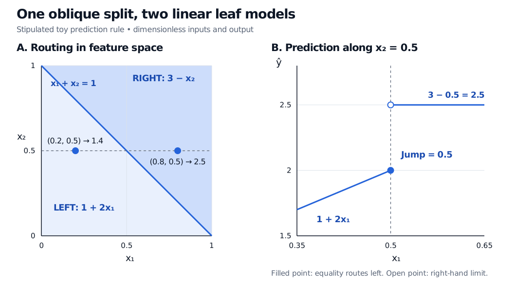
Stipulated toy tree on dimensionless features. The diagonal x1 plus x2 equals 1 separates a left leaf predicting 1 plus 2x1 from a right leaf predicting 3 minus x2. Point (0.2,0.5) predicts 1.4 and (0.8,0.5) predicts 2.5. Along x2 equals 0.5, equality at x1 equals 0.5 predicts 2, while the right-hand limit is 2.5: a jump of 0.5.

Original stipulated toy rule. Panel A shows routing; panel B holds x₂ at 0.5 to reveal a prediction jump despite linear leaf models. No fitted data or market performance is implied.

Linear within leaves does not guarantee continuity across leaves. Equality goes left under the stated rule. At

(0.5,0.5)

the prediction is

2

. Holding

x_2=0.5

and moving just to the right of

x_1=0.5

gives

2.5

, a jump of

0.5

. Continuity would require neighbouring formulas to agree along their shared boundary; this rule imposes no such constraint. Smoothing toward ancestor predictions need not enforce that agreement either.

More flexibility needs more evidence

An oblique split can express a combined feature condition compactly. Linear leaves can represent local slopes instead of flat predictions. The additional coefficients also create more opportunities for overfitting, especially when few observations reach a leaf or predictors are nearly collinear. Linear leaves can extrapolate outside their training feature range; that arithmetic does not establish a reliable economic relationship.

For a financial forecast, features must be available at the forecast time and training outcomes must already be observable. Fit feature transformations, split directions and thresholds, and leaf regressions using training data only. Choose complexity on separate validation data and preserve a final untouched test. If outcome windows overlap, the membership lesson on finance-aware validation, with a public preview, explains purging and embargoes.

The membership lesson Decision Trees: Splitting Criteria and Pruning, also with a public preview, develops the conventional baseline. Compare added geometry and local slopes against that baseline on the same eligible holdout observations. A compact diagonal rule is a representation advantage; any forecast advantage must be measured.

Sources

Murthy, Kasif and Salzberg (1994), A System for Induction of Oblique Decision Trees, §1 (split geometry) and §3.1 (OC1 search).
Quinlan (1992), Learning with Continuous Classes, §§1–2 (model trees, linear models, pruning and smoothing) and Figure 1 (single-attribute splits).

Two choices, four combinations

Route first, then evaluate the leaf

More flexibility needs more evidence

Sources

Related terms

Decision tree

Linear regression

Overfitting