Non-negative matrix factorisation: Definition & Examples

Non-negative matrix factorisation (NMF) approximates a nonnegative matrix by the product of two nonnegative matrices. Every reconstructed entry is a sum of nonnegative contributions. For a quant analysing filing word counts or trading volumes, this offers an additive description of activity; applying it directly to signed returns violates the input restriction.

With observations in rows and features in columns, write

V\approx WH,\qquad V\in\mathbb{R}_{\geq0}^{n\times p},\quad W\in\mathbb{R}_{\geq0}^{n\times k},\quad H\in\mathbb{R}_{\geq0}^{k\times p}.

Rows of

H

describe component patterns across features; rows of

W

give their observation-specific weights. Thus

(WH)_{ij}=\sum_{a=1}^{k}W_{ia}H_{aj}

. A component can contribute nothing, but cannot subtract another component away. The orientation here transposes the observation-column convention used in Lee and Seung's original paper.

Reading an exact product

Consider three fictional observations of two nonnegative features, measured in arbitrary dimensionless units. Supply these factors:

W=\begin{pmatrix}1&0\\0&1\\1&1\end{pmatrix},\qquad H=\begin{pmatrix}2&1\\1&3\end{pmatrix},\qquad V=WH=\begin{pmatrix}2&1\\1&3\\3&4\end{pmatrix}.

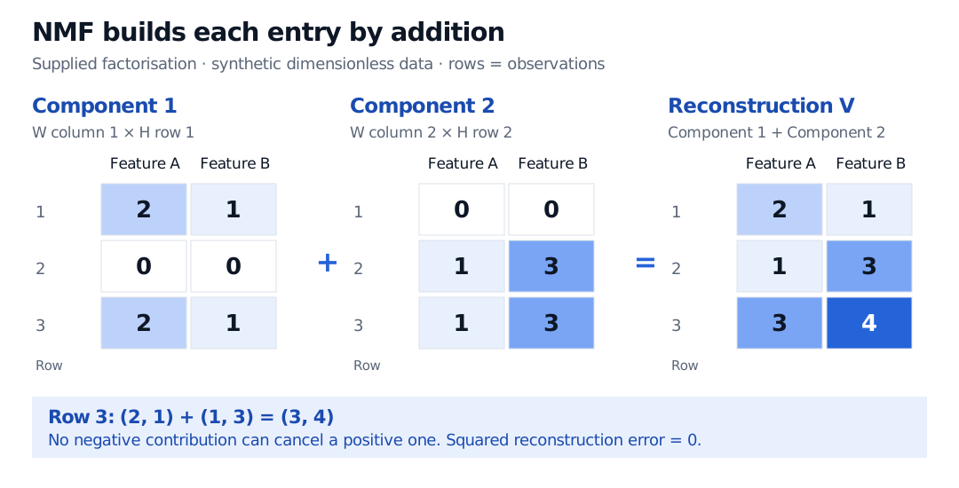
The first observation uses only the first pattern, $(2,1)$ ; the second uses only $(1,3)$ . The third uses one unit of each: $(2,1)+(1,3)=(3,4)$ . These are component weights, not probabilities: they need not sum to one.

Two synthetic dimensionless NMF contributions add entry by entry: component one has rows (2,1), (0,0), (2,1); component two has rows (0,0), (1,3), (1,3); their sum has rows (2,1), (1,3), (3,4). Squared reconstruction error is zero.

Original supplied-factor example. Each panel uses the same observation rows and feature columns. Numbers show additive contributions; shading encodes their nonnegative magnitude.

The squared reconstruction error is zero. The top two rows have determinant

2\cdot3-1\cdot1=5

, so

V

has matrix rank two. This tiny example illustrates multiplication, not data compression: its two factors contain ten entries, versus six in

V

. Nor did an optimiser discover these factors; they were supplied.

Even this perfect reconstruction does not identify their scale. Double the first column of $W$ and halve the first row of $H$ :

\widetilde W=\begin{pmatrix}2&0\\0&1\\2&1\end{pmatrix},\qquad \widetilde H=\begin{pmatrix}1&1/2\\1&3\end{pmatrix}.

Their product is still $V$ . Component reordering also preserves the product. A normalisation convention can fix this scale freedom without proving that the remaining representation is unique.

What fitting actually minimises

A common objective is squared Frobenius norm:

\min_{W,H\geq0}\;\lVert V-WH\rVert_F^2 =\min_{W,H\geq0}\;\sum_{i,j}\bigl(V_{ij}-(WH)_{ij}\bigr)^2.

Another is generalised Kullback–Leibler divergence, with $Q=WH$ :

D(V\Vert Q)=\sum_{i,j}\left[V_{ij}\log\frac{V_{ij}}{Q_{ij}}-V_{ij}+Q_{ij}\right].

Use

0\log(0/q)=0

; a positive observation reconstructed as zero gives infinite divergence. These objectives penalise discrepancies differently and can produce different fits. Joint optimisation in

W,H

is nonconvex; a decreasing objective does not certify a global optimum. Lee and Seung analyse separate multiplicative updates for the two losses.

Additive does not mean causal

The original parts-learning paper demonstrates image and text representations, while explicitly warning that nonnegativity alone is insufficient to recover meaningful parts from every dataset. An interpretable component label remains a hypothesis about the data, not evidence of an economic cause or statistical independence.

Negative returns cannot be reconstructed by $WH\geq0$ . Adding a constant to make them nonnegative changes what zero means and changes the decomposition problem. Using absolute returns instead asks about movement magnitudes and discards direction. Choose the representation for its intended meaning before interpreting the components.

For the unconstrained comparison, the SelfMadeQuant lesson The Eckart-Young Theorem explains the optimal truncated-SVD reconstruction at a given rank. Its preview is public; the full lesson requires membership. That theorem does not guarantee an optimal NMF solution with nonnegative factors.

Sources

Lee and Seung, Algorithms for Non-negative Matrix Factorization, Sections 2–4: factorisation, Euclidean and divergence objectives, nonconvexity and update rules. Presented at NIPS 2000; proceedings published in 2001.
Lee and Seung (1999), Learning the parts of objects by non-negative matrix factorization, pp. 788–790 and Figure 2: additive representations, limitations and scale invariance.

Reading an exact product

What fitting actually minimises

Additive does not mean causal

Sources

Related terms

Matrix

Matrix rank