A Gaussian mixture classifier can separate classes with identical means. Follow a checked Bayes example and distinguish labels, latent components and covariance constraints.
Mixture discriminant analysis
Mixture discriminant analysis (MDA) is a supervised classifier that represents each labelled class with a mixture of Gaussian feature distributions, then combines those densities with class priors to obtain class probabilities. It can distinguish classes whose observations occupy several separate regions, even when their overall means coincide. For a quant modelling a labelled liquidity condition, this allows different feature patterns to support the same label without compressing them into one representative observation.
The class labels are observed during training. The component memberships within each class are latent. Fitting clusters to an unlabelled pooled sample and naming them afterwards is a different procedure.
Here ϕp is the p-dimensional normal density, Rk is the component count for class k, and wkr is a within-class mixing weight. Every component in every class shares one positive definite covariance matrix Σ. The weights differ from the class priorsπk=P(Y=k), which sum to one across classes.
Sum the contributions of all components belonging to a class before comparing classes. Selecting the single most likely component and returning its parent label can give a different answer.
With one component per class, this construction reduces to linear discriminant analysis. With several components, the class boundary need not be linear despite the common component covariance. Allowing separate component covariances is another mixture-classifier specification; it should be stated explicitly rather than silently substituted for this construction.
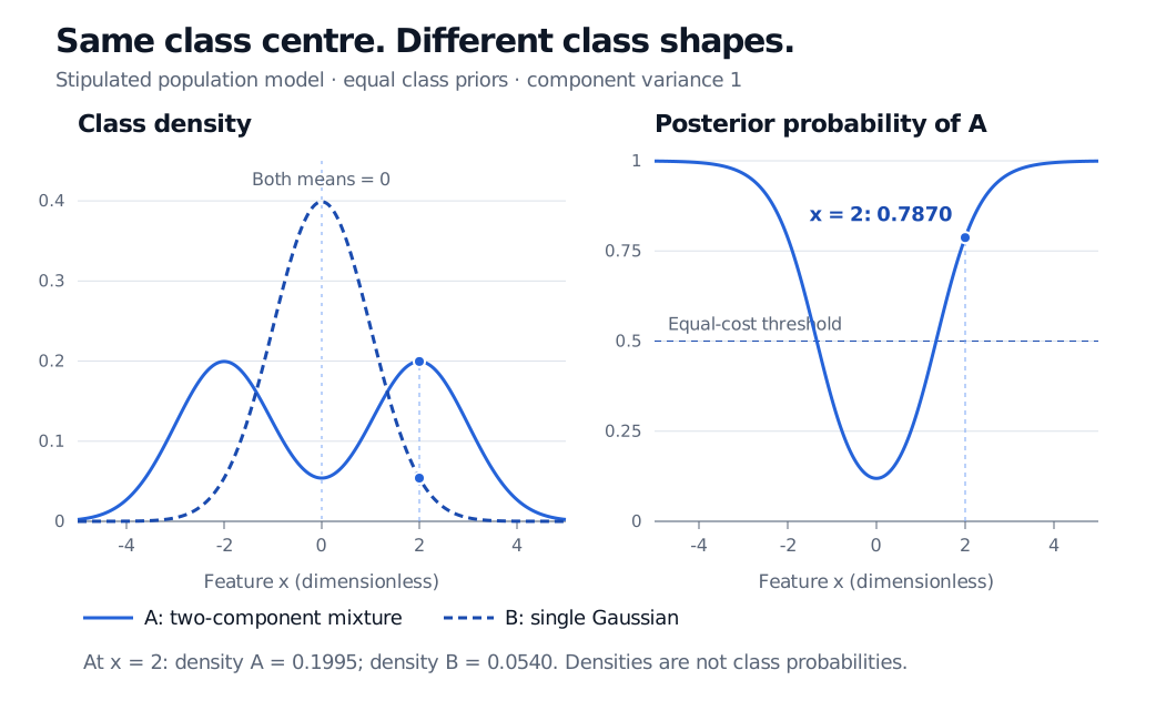
Both class means are zero; the prediction is not a tie
Consider a fictional population model, with a dimensionless feature X:
The second normal parameter is variance. All three component variances equal one. These parameters are stipulated; no observations were generated and no model was fitted.
Class A has mean 21(−2)+21(2)=0, the same as class B. A population LDA model with these identical means, a common covariance and equal priors ties everywhere. The mixture model retains information that those means discard: A has two concentrations away from the centre, while B concentrates at the centre.
Writing ϕ for the standard normal density, at x=2:
Equal priors cancel in the ratio. Under equal misclassification costs, predict A. The density 0.1995 is not a 19.95% class probability: the posterior requires normalising the prior-weighted densities across the possible labels. By symmetry, x=−2 gives the same class posterior; a large negative feature can support A just as a large positive one does.
Stipulated class A mixes normals centred at minus 2 and plus 2 with equal weights; class B is standard normal. Both means are zero. At x equals 2, densities are 0.1995 and 0.0540, giving posterior A 0.7870 under equal class priors.
Original analytic illustration of the stipulated distributions. The left panel shows class densities; the right shows their Bayes posterior. The dashed probability threshold assumes equal error costs.
What fitting adds—and what it does not establish
The expectation-maximisation algorithm can fit the hidden component structure. For an observation whose known label is k, its E-step responsibilities are normalised within that class, not across every class. The M-step updates component means and mixing weights from those soft assignments and pools weighted component residuals to estimate the shared covariance. The original paper, §2 and §2.1, describes this procedure and its initialisation.
A component is a density-building device, not evidence of a true economic regime. One labelled condition can need several components, and their numbering has no economic meaning. MDA also does not impose persistence or transition probabilities between dates.
Component counts and starting values affect the fit. More components offer flexibility but also more opportunity to fit noise. If separate component covariances are allowed, small components can develop singular covariance estimates; the official Gaussian-mixture guide discusses this estimation problem. Record covariance constraints and regularisation along with the counts.
For market data, choose these settings using training and validation windows that respect information availability. Keep preprocessing and fitting inside each training window; a future-return label is usable only after its outcome is observed. Compare held-out class errors and probability calibration. A richer density or a confident posterior alone establishes neither calibrated forecasts nor a profitable trading rule.
For the fitting mechanics, Mixture of Gaussians and the EM Algorithm derives soft component responsibilities and their weighted updates. Its preview is public; the full lesson requires membership. That lesson allows component-specific covariances, so reproducing the MDA construction here requires the shared covariance constraint.