A mixture density network predicts an input-dependent distribution. See why component variances of 1 can produce total variance 4, and how density training differs from mean regression.
Mixture density network
A mixture density network (MDN) is a neural network whose outputs specify the parameters of a mixture distribution, conditional on its inputs. It predicts a distribution for a continuous target rather than only a point forecast. For a quant forecasting a future return, that distinction allows several concentrations of possible outcomes to remain visible instead of being compressed into one average.
What comes out of the network
For a scalar target Y and input features x, a Gaussian MDN represents the conditional density as
pθ(y∣x)=k=1∑Kπk(x)N(y;μk(x),σk2(x)).
Here N(y;μ,σ2) denotes a normal density evaluated aty. Its second parameter is variance; σ is standard deviation. The network produces mixing weights, means and scales, all of which can change with the input. A fixed set of Gaussian parameters fitted to an unconditional sample is a different specification.
Weights must be nonnegative and sum to one; scales must be positive. Bishop’s original paper, §3, uses softmax for weights, unrestricted outputs for means and exponentials for scales. With finite logits, softmax gives strictly positive weights. A Gaussian MDN with a scalar target needs 3K raw outputs under this parameterisation, although the normalised weights have only K−1 degrees of freedom.
A mean of 3 is not the whole forecast
Suppose that at one fixed input x0, a fictional network supplies
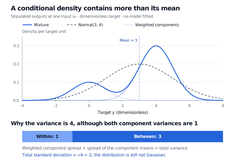
Y∣x0∼0.25N(0,1)+0.75N(4,1).
The target is dimensionless. These are stipulated outputs: no training sample was generated and no network was fitted. Sampling from this forecast means selecting component 1 with probability 0.25 or component 2 with probability 0.75, then drawing from that component’s normal distribution. It does not mean averaging two independent normal draws.
The conditional mean is
m=0.25(0)+0.75(4)=3.
The variance includes the spread within components and the spread of their means:
Thus the predictive standard deviation is 2, even though each component’s standard deviation is 1. Reporting the weighted component variance, 1, would discard three quarters of the total variance in this example.
Stipulated mixture at one input: weights 0.25 and 0.75, means 0 and 4, and component variances 1 and 1. Its density differs from a normal with mean 3 and variance 4. Within-component variance 1 plus between-component variance 3 equals total variance 4.
Original analytic illustration of stipulated outputs, with no fitted data. The dotted curves are weighted component densities; the solid curve is their sum. The dashed Gaussian matches only the mixture’s mean and variance.
The mixture is notN(3,4). For example, its density at zero is approximately 0.099836, whereas the matching Gaussian’s density there is 0.064759. Equal means and variances do not imply equal distributions, tail probabilities or quantiles. Nor does a two-component mixture always have two modes: overlap and weights determine the shape.
Gradients propagate through the mixture parameters into the network. Minimising squared error between yi and the mixture mean instead would leave different density shapes with the same mean indistinguishable to the loss.
Compute each log density by applying log-sum-exp to the terms logπk+logN(y;μk,σk2). Exponentiating very negative component log densities first can underflow to zero; the SciPy log-sum-exp documentation describes the stable calculation.
Positive scales alone do not prevent them becoming arbitrarily small. A narrow component placed on an observation can inflate its density; Gaussian-mixture likelihoods can develop singularities. Scale floors or regularisation, initialisation and component count therefore matter. State the scale convention and constraints when reporting a fit.
For financial forecasts, inputs must be available at the forecast origin, and training labels must have completed by the training cutoff. Assess held-out density scores and interval coverage through time. Mixture components need not be economic regimes, and predictive spread from one fitted MDN does not by itself measure uncertainty about the fitted network’s parameters. A flexible density is no guarantee of reliable tail forecasts.
For the simpler baseline, The Probabilistic Interpretation of Least Squares derives why fixed-variance Gaussian likelihood yields squared-error regression. Its preview is public; the full lesson requires membership.