Compare relative triplet margins, cosine similarity thresholds and Euclidean pair losses, with worked examples and financial label and validation boundaries.
Triplet loss and cosine embedding loss
Triplet loss trains a representation so that an anchor is closer to a designated positive example than to a negative example by a margin. Cosine embedding loss trains pairs using the angle between their vectors: similar pairs should align, while dissimilar pairs should stay below a chosen similarity threshold. Both are metric-learning objectives. In quantitative research, they can shape a representation used to retrieve comparable disclosures or market episodes—but the meaning of “comparable” comes from the training labels, not from the loss itself.
A neural network maps an input x to an embedding fθ(x). A loss function then scores relationships among those embeddings. These objectives train geometry rather than directly forecasting returns. A low training loss is not evidence of useful out-of-sample neighbours or trading performance.
Triplets enforce a relative ordering
Write a, p and n for the anchor, positive and negative embeddings. A common triplet objective is
Ltriplet=max{0,d(a,p)−d(a,n)+α},α>0.
It is zero when the negative is at least α farther from the anchor than the positive is, using the specified distance function d. Merely putting the negative farther away is insufficient when the gap is smaller than the margin. Conversely, zero loss need not put the positive at the anchor: it constrains a relative gap.
The FaceNet paper, Section 3.1, uses squared Euclidean distance and unit-normalised embeddings. The current PyTorch TripletMarginLoss documentation instead specifies a norm distance, unsquared by default, with a numerical-stability adjustment. Those conventions are not interchangeable.
Consider an exact, one-dimensional toy with anchor 0, positive 1, negative 1.5 and margin 1. These are unnormalised synthetic coordinates, not FaceNet's unit-sphere setup. Ignoring numerical-stability adjustments:
Distance convention
Positive distance
Negative distance
Triplet loss
Euclidean
1
1.5
max(0,1−1.5+1)=0.5
Squared Euclidean
1
2.25
max(0,1−2.25+1)=0
The numerical margin “1” has different units in these two rows. Changing to squared distances while retaining the same number changes the constraint; it is not a harmless implementation detail.
Which triplets enter training also matters. Easy triplets already outside the margin contribute zero loss. Mining selects informative positives or negatives, but the hardest negatives may be mislabelled or unrepresentative. FaceNet's Section 3.2 discusses this problem and semi-hard negatives: farther away than the positive, yet still within the required margin. This is a sampling choice, not a guarantee that the learned neighbours are economically meaningful.
Cosine embedding loss sets an angular threshold
For two nonzero embeddings u and v, let
s=∥u∥2∥v∥2u⊤v.
Cosine similarity s lies between −1 and 1. Using the label convention in PyTorch CosineEmbeddingLoss, the per-pair loss is
Here m is a similarity ceiling for negative pairs, not a required distance gap between two pairs. With margin m=0.2, a negative pair stops contributing as soon as its cosine similarity is at most 0.2. It need not point in the opposite direction.
For synthetic unit vectors u=(1,0) and v=(0.6,0.8), the cosine similarity is 0.6. The similar-pair loss is 1−0.6=0.4; the dissimilar-pair loss at margin 0.2 is 0.6−0.2=0.4. The equal losses arise from these chosen numbers; the label tells training which relationship to encourage.
Multiplying either nonzero vector by a positive scalar leaves cosine similarity unchanged. That can help when direction matters and magnitude is a nuisance. It can discard useful information when magnitude carries economic meaning, such as order size. A zero vector has no mathematical cosine direction; numerical safeguards in software do not supply one.
For unit vectors, squared Euclidean distance equals 2(1−s). Thus angular and Euclidean geometry are connected after normalisation, but the pairwise and triplet objectives still impose different constraints and use different margin conventions.
A third objective: pairwise Euclidean contrastive loss
“Contrastive loss” can name several objectives within contrastive learning. To distinguish the mechanisms, define this pairwise Euclidean version, with d the distance between embeddings, y=1 for similar and y=0 for dissimilar:
Lpair=yd2+(1−y)max(0,M−d)2.
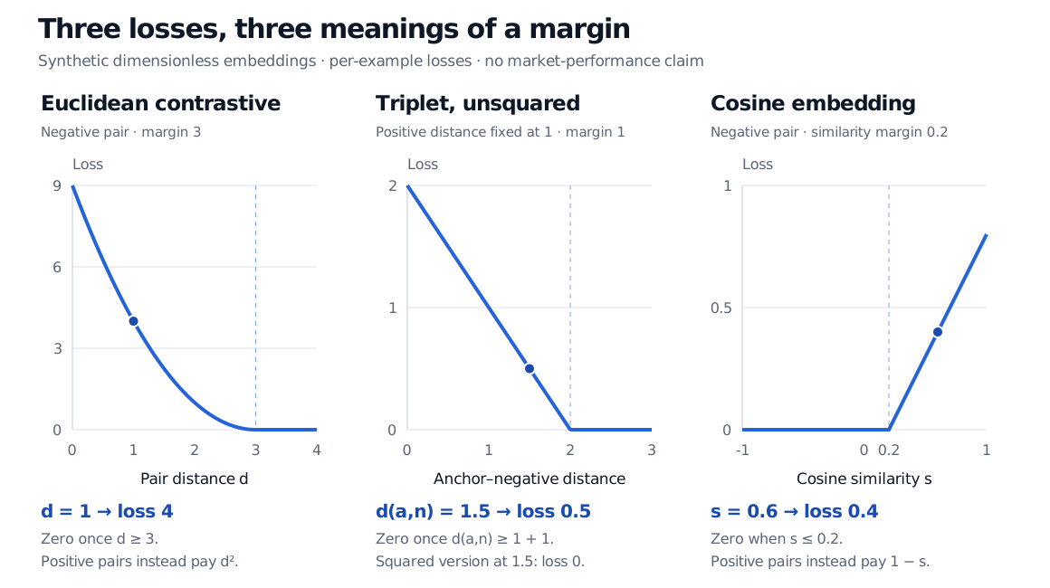
There is no factor of one-half here. At margin M=3, a positive pair at distance 2 costs 4; a negative pair at distance 1 also costs 4; a negative pair at distance 4 costs zero. Positive pairs are pulled together without a positive-pair dead zone, while negatives stop contributing once they reach the absolute distance boundary.
The official Keras Siamese contrastive example implements this form with the opposite binary coding: 0 means matching and 1 means nonmatching. Reverse its labels to obtain the equation above. Check label meanings before transferring data or formulas between implementations.
Three synthetic loss curves: a Euclidean contrastive negative pair with margin 3 has loss 4 at distance 1; an unsquared triplet with positive distance 1 and margin 1 has loss 0.5 at negative distance 1.5; a cosine negative pair with margin 0.2 has loss 0.4 at similarity 0.6.
The Euclidean pair margin is an absolute distance boundary, the triplet margin is a relative distance gap, and the cosine margin is a similarity ceiling. All examples are synthetic.
Financial labels define what the geometry learns
A disclosure-retrieval task might define positives as two passages about the same accounting topic and negatives as passages about other topics. That definition trains topical similarity. It does not train similarity of future returns or identify comparable issuers for valuation without additional evidence. Sector membership, shared vocabulary and overlapping market windows can also create easy shortcuts that fail in the intended application.
Choose the evaluation split before constructing training pairs or mining negatives. Keep held-out observations out of training tuples and fit the encoder and learned preprocessing within the training window. General training-only transformation guidance appears in scikit-learn's data-leakage discussion.
If similarity labels depend on later outcomes, they become available only after those outcomes are observed. A historical fit must use completed labels available by its cutoff; retrieving past windows does not justify training the encoder on future outcomes. Otherwise the representation itself introduces look-ahead bias. Overlapping outcome windows also require appropriate separation. The Time-Ordered Train, Validation and Test Design lesson develops those eligibility and pipeline boundaries (public preview; full lesson requires membership).
Evaluate the intended retrieval or downstream task in later held-out periods, and hold out issuers too when deployment must handle new identities. Report the label rule, distance convention, normalisation, margin, mining procedure and loss reduction. A smaller loss under a different convention is not a fair model comparison.