Understand how observed-price noise contaminates high-frequency realised variance, why finer sampling can worsen a naive estimate, and what noise-aware methods assume.
Market microstructure noise
Market microstructure noise is the difference between an observed market price and a model's latent efficient price arising from the trading and observation process. It matters when estimating realised volatility: adding more intraday observations can add more noise variation, rather than produce a better estimate of the underlying price variation.
“Noise” does not mean the transaction was erroneous. An ask-side execution is a real price paid. The distinction concerns the quantity being estimated: the variation of an unobserved efficient price, rather than every movement between executable transaction prices. A quote midpoint is a useful alternative observation, but is not automatically the efficient price. Hansen and Lunde's original analysis defines noise relative to a latent log-price and also discusses effects introduced by constructing a sampled price series.
Several mechanisms, different assumptions
Bid–ask bounce: transactions switch between bid and ask, creating reversals even when the underlying efficient price is unchanged.
Price discreteness: a tick size forces observed prices onto a grid. Rounding error need not be independent of the price being rounded.
Price adjustment and observation timing: quotes or sampled previous trades can lag an efficient-price change. The resulting discrepancy can depend on efficient returns and on past observations.
These mechanisms need not produce independent, identically distributed errors. In particular, endogenous noise is statistically related to the efficient-price process. Hansen and Lunde report both dependence over time and correlation with efficient-price increments in their historical equity study; this is evidence against treating independent noise as a universal description. Their findings concern their sample, rather than a fixed law for every asset and venue. The September 2004 manuscript linked here precedes the 2006 journal article.
The Spread Measurement lesson develops the bid–ask reversal mechanism through the Roll model and distinguishes spread measures. Its preview is public; the full lesson requires membership.
A return contains two noise observations
Write observed log prices, at fixed times t0,…,tn, as
Yi=Xi+ϵi,ΔYi=ΔXi+ϵi−ϵi−1.
Here Xi=Xti is the efficient log price. Noise is additive in log units, not currency units. For the following calculation assume X is a square-integrable continuous martingale, and the n+1 errors are independent and identically distributed, have mean zero and variance η2, and are independent of X.
The cross-term has expectation zero. Each differenced noise term has variance 2η2. For this martingale on a fixed grid, the expected efficient squared-increment sum equals expected quadratic variation, so
E[RVY]=E[[X]T]+2nη2.
The bracket [X]T denotes efficient-price quadratic variation. For a continuous diffusion it is integrated variance, ∫0Tσt2dt. The equality above is an expectation under the stated model, not an identity between one day's sampled returns and that day's integrated variance. A drift or other noise assumptions require their own treatment.
Although the level errors are independent here, their differences share an observation with opposite signs:
Cov(ϵi−ϵi−1,ϵi+1−ϵi)=−η2.
Thus independent price noise does not imply independent return noise. This additive observation setup is the starting point of Zhang, Mykland and Aït-Sahalia's two-scales paper, whose original latent price is a continuous Itô process with independent noise.
One fixed day: 2% becomes a 4.899% benchmark
Consider an illustrative day with expected efficient quadratic variation 0.0004, whose square root is 2%. Let noise standard deviation be η=0.001 log units, and use 1,000 return increments from 1,001 price observations, including both endpoints.
E[RVY]=0.0004+2(1000)(0.001)2=0.0024.
The expected noise contribution, 0.0020, is five times the expected efficient contribution. Taking the square root of the expected total gives
E[RVY]=0.0024≈0.0489898=4.89898%.
This square root of expected realised variance is neither a realised estimate from market data nor the expected realised volatility E[RVY]. The square root is nonlinear; those expectations cannot be interchanged. Neither percentage is annualised.
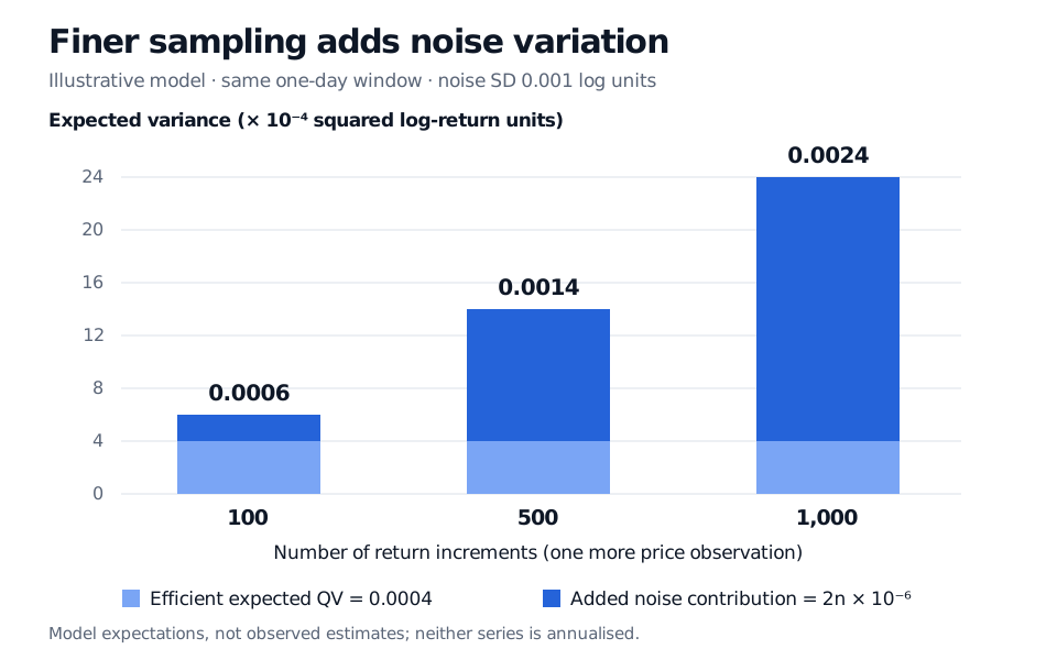
Expected realised variance is 0.0006 with 100 increments, 0.0014 with 500 and 0.0024 with 1000. Expected efficient quadratic variation remains 0.0004; the growing remainder is observation noise.
Illustrative model expectations over the same day, with independent noise SD 0.001 log units. More increments increase the noise contribution while expected efficient variation stays fixed.
Use the fine data with an appropriate estimator
Sparse sampling can reduce noise contamination but uses less information about the path. There is no universally best sampling interval. The two-scales method averages variance sums on slower subgrids and uses the fine-grid sum to correct their noise contribution. That is more structured than declaring the noisiest observations worthless; its validity depends on the observation model and sampling assumptions. See the original paper's §§1.2 and 2.1.
Realised kernels instead combine the variance sum with weighted return autocovariances. Barndorff-Nielsen, Hansen, Lunde and Shephard's original research report, §§2 and 5, starts with independent white noise and then analyses specified forms of serial dependence and endogeneity. Kernel choice, bandwidth and boundary treatment matter; robustness to those specified models is not robustness to arbitrary contamination.
Even the elementary bias expression changes when assumptions change. For stationary, zero-mean level noise independent of X, let γ0=Var(ϵi) and γ1=Cov(ϵi,ϵi−1). The expected noise contribution becomes 2n(γ0−γ1). With endogenous noise, the cross-term can also survive. Subtracting a guessed constant from every realised-variance calculation therefore does not solve the general problem. Removing expected bias alone is also different from making estimation error shrink.
Before interpreting a high-frequency estimate, name the price series, sampling clock, estimator and noise assumptions. Cleaning a bad timestamp and estimating variation in a valid but noisy transaction series address different problems.
Hansen and Lunde, Realized Variance and Market Microstructure Noise, September 2004 manuscript, Introduction and §2, including Lemma 1; journal publication 2006 — latent versus observed prices, sampling and independent-noise benchmark, with historical evidence challenging independence.