Read training and validation error against sample size, distinguish it from epoch loss, and build time-aware curves without leaking future financial data.
Learning curve
A learning curve plots a model's training and validation performance against the number of observations used to fit it. For a quant researcher, it helps frame a practical question: is weak prediction plausibly a shortage of useful training data, or should the model, features or fitting procedure change?
Here, the horizontal axis is training sample count. An optimisation curve instead plots loss against epochs or parameter-update steps on a given dataset. Both are sometimes called learning curves, so always inspect the axis. A validation curve against a hyperparameter, such as regularisation strength, answers another question again.
A shrinking gap, with no promise attached
Consider an invented forecasting exercise. All errors are mean squared error (MSE), measured in the same squared target units; lower is better. Keep the target, features, model settings, fitting budget and validation observations fixed while changing the training subset size.
Training observations
Training MSE
Validation MSE
Validation minus training
100
1.0
5.0
4.0
400
2.0
3.5
1.5
1,600
2.5
3.0
0.5
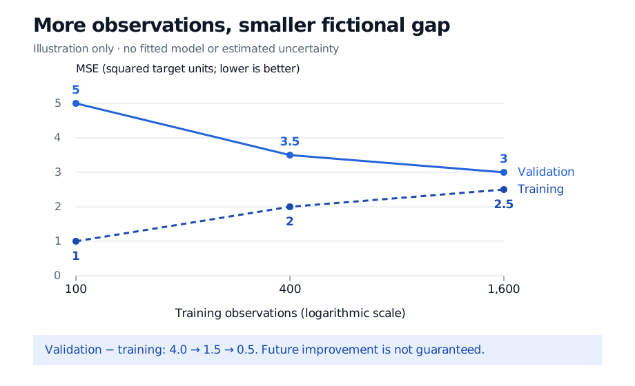
Fictional MSE in squared target units at training sizes 100, 400 and 1600: training errors 1, 2 and 2.5; validation errors 5, 3.5 and 3; gaps 4, 1.5 and 0.5. The sample-count axis is logarithmic.
Original fictional sample-size learning curve. Connecting lines guide the eye; no model was fitted and no uncertainty bands are estimated.
At 100 observations the model fits its own data much better than held-out data. This is consistent with overfitting. In the fictional table, adding observations narrows that gap even though training error rises: fitting more observations leaves less freedom to accommodate each one. The validation error is the relevant improvement here.
These three points do not prove that the next batch will improve performance, that either curve must be monotone, or that their eventual meeting point will be useful. Nor does the observed gap equal the variance term in a bias-variance decomposition. It is a diagnostic comparison, not an identification of the error components.
If both errors stay high and close together, underfitting, weak features or a fitting failure deserve investigation. A small gap alone cannot distinguish these explanations from substantial outcome noise. Judge the error level against a relevant baseline; agreement between two poor curves is no success criterion.
Construct the experiment inside the information boundary
For each chronological validation block, choose nested training subsets entirely before that block, with labels already available at fit time. For example, predeclare successively longer trailing windows ending at the same eligible cutoff. Record the window rule: changing sample count also changes the historical regimes represented.
Refit the whole pipeline on each subset. Scaling, imputation and feature selection must learn only from that subset, followed by model fitting. Applying a scaler estimated once on the largest sample to every smaller fit would give the small-sample experiment information it was not meant to have. Keep hyperparameter selection inside the development procedure too.
Repeat across suitable time blocks and, where relevant, fitting seeds. Report the individual block results and dispersion when available, with the meaning of any error bars stated. A standard deviation across overlapping folds is not automatically a confidence interval for future performance. The fictional table supplies no repetitions, so its figure has no empirical error bars.
Financial observations are often dependent. Overlapping outcome horizons can transmit label information across a boundary; chronology alone does not settle that issue. Check label intervals and remove conflicting training labels where necessary. Adding older market history may introduce a different regime rather than more comparable evidence. Raw row count therefore does not mean independent information, and there is no universal conversion to an “effective sample size.”
The time-ordered validation lesson develops these information and refitting rules (full lesson requires membership; public preview available).
Keep validation separate from final assessment
The held-out observations used to inspect this curve are a validation set: they inform research choices. Reserve an untouched test set for assessing the frozen procedure. Repeatedly adapting to that final test turns it into further selection data.
In scikit-learn, learning_curve varies training sizes within cross-validation splits. Its API calls held-out fold results “test scores”; when those results guide choices, their role is validation. Supply an appropriate splitter for temporal data: leaving shuffling off does not by itself make ordinary K-fold evaluation chronological. Check the scoring convention too; negative-MSE scores must have their sign reversed when displayed as positive MSE losses.
If the horizontal axis is epochs, use the loss-curve diagnosis lesson to investigate optimisation and checkpoint selection (full lesson requires membership; public preview available).