Replace a large kernel matrix with explicit features. Compare landmark-based Nyström projection with Fourier sampling, and see exactly what a rank-one approximation loses.
Nyström approximation and random Fourier features
Nyström approximation and random Fourier features construct small, explicit feature vectors whose inner products approximate a chosen kernel. They make nonlinear kernel methods usable with linear-model solvers. For a quant fitting execution costs across many orders, the practical attraction is replacing a large table of pairwise order similarities with a manageable table of transformed inputs.
Write the training Gram matrix as Kij=k(xi,xj). A feature matrix Z has one row z(xi)⊤ per observation and aims for
K≈ZZ⊤,k(x,x′)≈z(x)⊤z(x′).
If there are n observations and r features, storing Z takes nr entries instead of n2 for a dense K. This saves memory when r≪n; it does not promise that the resulting predictions match an exact fit. scikit-learn, Kernel approximation
Here C is n×m, W is m×m, and W† is the Moore–Penrose pseudoinverse. It equals the inverse when W is nonsingular. Duplicate or dependent landmark features can make W singular; an ordinary inverse then does not exist.
If W=U+Λ+U+⊤ retains all its strictly positive eigenvalues, an explicit factor is
Z=CU+Λ+−1/2,z(x)⊤=k(x,L)U+Λ+−1/2.
The second expression transforms a new input using the same landmarks and normalization. In feature-space terms, this projects onto the span of the landmark feature vectors. It is data dependent even when the landmarks are sampled randomly. The classical construction and its projection interpretation are developed in Rasmussen and Williams, §8.1, following Williams and Seeger (2001).
Truncation and regularization change the approximation. Dropping small positive eigenvalues gives a truncated pseudoinverse. Replacing W† by (W+ηI)−1, with η>0, gives a regularized variant. Neither is the exact all-positive-eigenvalue projection above. State the threshold or η rather than silently treating all three constructions as identical.
A landmark can reproduce similarities and still lose length
Consider a fictional, dimensionless example:
K=(10.50.51).
This matrix is positive definite: its eigenvalues are 1.5 and 0.5. Select the first observation as the sole landmark. Then
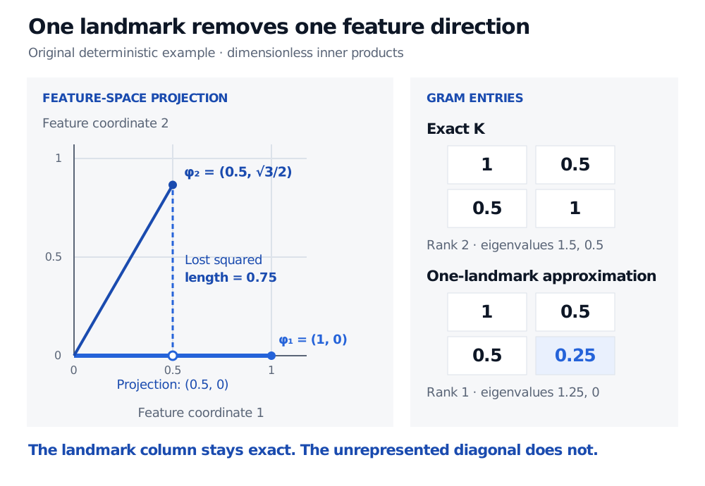
C=(10.5),W=(1),K=CC⊤=(10.50.50.25).
The first row and column are exact, but the second diagonal falls from 1 to 0.25. Its error is 0.75. The approximation has rank one, with eigenvalues 1.25 and 0; the original has rank two.
The geometry explains the missing amount independently. Choose exact feature vectors
ϕ1=(1,0)⊤,ϕ2=(1/2,3/2)⊤.
Their inner products give K. Projection onto the first landmark removes the second coordinate of ϕ2. The lost squared length is (3/2)2=3/4. Thus the residual is
K−K=(0000.75).
Exact unitless feature vectors are phi1 equal to (1,0) and phi2 equal to (0.5, square root of 3 divided by 2). Projecting onto the first landmark leaves phi2 with squared length 0.25 instead of 1. The omitted squared perpendicular length is 0.75; the approximate Gram matrix has rank 1.
Original deterministic geometry for the two-observation example. The first landmark retains the horizontal feature direction and discards the vertical direction. Matrix entries are dimensionless inner products.
This is a controlled loss of feature directions, not an identity for the full kernel. In particular, an exact landmark column does not establish a good approximation for the rest of the sample. Dividing the approximate rows by their norms would also change the approximating kernel.
Random Fourier features: sample the kernel's spectrum
Random Fourier features (RFF) use a different construction. For a continuous, real, stationary PSD kernel on Rd, write k(x,x′)=κ(x−x′). With κ(0)=1, Bochner's theorem provides a spectral probability measure p satisfying
κ(δ)=Eω∼p[cos(ω⊤δ)].
Draw r independent frequencies ωj∼p and independent phases bj∼Uniform[0,2π]. One real-valued map is
zj(x)=r2cos(ωj⊤x+bj),E[z(x)⊤z(x′)]=k(x,x′).
For the Gaussian kernel k(x,x′)=exp(−∥x−x′∥2/(2ℓ2)), draw ωj∼N(0,ℓ−2Id). An overall kernel amplitude a>0 requires multiplying the normalized map by a. This is Fourier sampling, not landmark selection. Rahimi and Recht, §3
The equality holds in expectation over draws. A finite realized map has error; increasing the feature count need not improve every pair monotonically. Its Gram matrix is PSD because it is ZZ⊤, though individual estimated similarities can be negative. Standard RFF requires stationarity; Nyström can also approximate nonstationary PSD kernels. The paired sine/cosine map in the paper's Algorithm 1 is another valid construction, with different feature-count bookkeeping.
Keep the approximation inside the research split
Choice
Nyström
Standard RFF
What fixes the coordinates?
Landmark inputs and their kernel matrix
Kernel spectrum and sampled frequencies/phases
Dependence on observed input values
Direct
None for a fixed kernel and input dimension
Main approximation budget
Landmark count and retained eigenvalues
Number of sampled features
What must travel with the fitted model?
Landmarks, kernel settings and normalization
Frequencies, phases and kernel settings
Both also need any fitted input preprocessing. In a chronological experiment, fit scaling and select Nyström landmarks using the training window only. Apply those frozen transformations to validation and test observations. Tune bandwidth, feature count and any eigenthreshold or regularization inside the training/validation procedure; selecting them from final test results leaks information. scikit-learn, §§12.1–12.2.1
Fix and record random seeds for reproducibility, and examine sensitivity across seeds without choosing the best seed on the final test set. RFF frequencies are data independent conditional on the kernel, but a bandwidth or scaler estimated using future inputs is still a data-dependent choice. Re-sampling frequencies at prediction time changes the coordinates under an already fitted model.
A linear ridge regression on Z is kernel ridge regression for the approximating kernel k(x,x′)=z(x)⊤z(x′), under matched loss, penalty and intercept conventions. Compare its held-out loss and operational cost with an exact-kernel benchmark when feasible; kernel approximation error alone is not a trading-performance measure.