Calculate IRR as the rate that makes signed cash-flow NPV zero, then see why one project can have two IRRs and why timing, conventions and scale matter.
Internal rate of return
The internal rate of return (IRR) is a discount rate that makes the net present value of a signed cash-flow schedule equal to zero. Payments made by the investor are negative; receipts are positive. IRR is a rate implied by those amounts and dates. It does not supply the cash-flow forecast, choose the appropriate required return, or measure risk by itself.
For evenly spaced periods, write
0=NPV(r)=k=0∑n(1+r)kCk,
where C0 is today’s cash flow and r is the effective rate per cash-flow period. The usual positive-growth-factor domain is r>−1. With yearly periods, the solved rate is annual effective; with monthly periods, it is a monthly rate.
The calculation builds on present value and net present value. OpenStax’s IRR chapter develops the zero-NPV idea and explains why a cash-flow schedule may have multiple solutions.
First, a schedule with a single answer
In a fictional equipment project, Mina’s team pays 10,000 USD now and expects net receipts of 6,000 USD after one year and 6,000 USD after two years. Assume those amounts occur as stated, with no additional fees or taxes.
Time
Net cash flow, USD
Today
−10,000
One year
+6,000
Two years
+6,000
The IRR solves
−10,000+1+r6,000+(1+r)26,000=0,
giving r≈13.066239% effective annually. Discounting the two receipts at that rate gives a combined present value of 10,000 USD, offsetting the initial outflow.
This is not the 20% undiscounted cash profit divided by two years. The first receipt arrives a year earlier than the second. IRR uses that timing rather than spreading the total cash profit evenly over the horizon.
Here there is one initial outflow followed only by positive receipts. Their discounted value falls continuously as the rate increases, so there is one admissible IRR. That useful property depends on the cash-flow pattern; a calculator’s single output does not establish it for every project.
At an assumed required return of 8%, this schedule has
For this conventional schedule, the IRR exceeding the required return corresponds to positive NPV. The next case shows why that comparison needs its assumptions.
A later payment changes the root problem
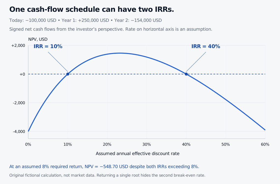
Mina then reviews a separate fictional pilot facility. It costs 100,000 USD today, produces 250,000 USD of net receipts after one year, and requires a 154,000 USD shutdown payment after two years. The last cash flow is an outflow, not another receipt.
NPV(r)=−100,000+1+r250,000−(1+r)2154,000.
Both 10% and 40% make this NPV zero. To see both roots directly, multiply the zero-NPV equation by (1+r)2 and factor:
−100,000(r−0.10)(r−0.40)=0.
There are two valid break-even rates. Neither is an arithmetic mistake.
Assumed annual-effective discount rate
NPV, USD
0%
−4,000.00
8%
−548.70
10%
0.00
25%
+1,440.00
40%
0.00
50%
−1,777.78
The pilot facility’s NPV curve crosses zero twice, at 10% and 40%. With an assumed 8% annual-effective discount rate it has negative NPV of 548.70 USD despite both IRRs exceeding 8%.
Original fictional project. Cash amounts and dates stay fixed. The curve shows NPV under different assumed discount rates, not observed returns or a forecast of market rates.
At an 8% required return, both IRRs exceed 8%, but NPV is negative. The usual shortcut fails because the later outflow makes the NPV profile non-monotonic. Selecting whichever root looks more attractive cannot change the cash flows.
Mixed signs do not even guarantee that a real IRR exists. For example, the yearly schedule −100, +50, −100 has negative NPV for every r>−1. Multiplying by (1+r)2 gives a quadratic with negative discriminant, so there is no real zero. A failed numerical search and a genuinely absent root are different possibilities.
A numerical answer needs a residual and a time unit
Many schedules require numerical root finding. Check a returned rate by substituting it into the NPV equation. The residual should be small relative to the cash amounts. Then inspect whether other admissible roots exist.
A bisection search finds a root inside a sign-changing bracket. It does not prove that there are no roots outside that bracket, and a root that merely touches zero need not create a sign change. A single initial guess can therefore conceal useful information. Microsoft’s IRR documentation describes its regular-period input convention, iterative search and optional initial guess.
Timing is just as important. With irregular dates, use explicit year fractions, for example
0=i∑(1+r)τiCi,
where the chosen convention defines τi as years from the valuation date. Do not pretend that unevenly dated receipts are equally spaced. Microsoft’s XIRR documentation describes its particular 365-day-based date calculation; that implementation is not a universal day-count rule for every market instrument.
For a monthly periodic IRR, the equivalent effective annual rate is (1+rmonth)12−1. Multiplying a monthly rate by 12 gives a nominal annual quotation, not the effective annual rate. The interest-rate article explains these conventions.
What IRR can tell a quant—and what it leaves out
A yield to maturity is a bond-specific IRR: it uses the full purchase price and the remaining promised coupon and principal payments, then applies the instrument’s quoting convention. The same root idea appears in money-weighted return, where deposits, withdrawals and terminal value determine the investor’s dated schedule.
Computing IRR requires no reinvestment-rate input. Turning interim receipts into a final pot of wealth requires additional assumptions about what happens to them. The YTM example shows that cash-flow IRR and terminal compound growth can differ.
A forecast IRR also depends on the forecast being right. It does not adjust automatically for uncertainty, funding needs or the appropriateness of the hurdle rate. When comparing alternatives, a higher IRR can accompany a smaller NPV because scale and timing differ. Use the signed cash flows and the appropriate valuation assumptions rather than ranking percentages alone.
For the bond application, read SelfMadeQuant’s YTM explanation, including its repricing check and convention conversion. The Bonds and Yields lesson gives a guided introduction to that cash-flow equation. Its public page is a preview; the full lesson requires membership.
Sources
Frank J. Fabozzi, Bond Markets, Analysis, and Strategies, 9th ed., Chapter 3: yield as the internal rate of return of dated investment cash flows.