Instrumented principal component analysis: Definition & Examples

Instrumented principal component analysis (IPCA) estimates latent factors while using observable characteristics to model assets' changing factor exposures. It lets a quant ask whether changing company attributes explain changing exposure to common return movements, rather than estimating a separate unrestricted loading for every asset at every date. Kelly, Pruitt and Su developed the approach in their asset-pricing research.

The fixed object is the map

In a basic return specification, let $z_{i,t}$ contain $L$ characteristics known at date $t$ , including any constant characteristic. With $K$ latent factors,

\beta_{i,t}=\Gamma^\top z_{i,t},\qquad r_{i,t+1}=\beta_{i,t}^\top f_{t+1}+e_{i,t+1} =z_{i,t}^\top\Gamma f_{t+1}+e_{i,t+1}.

The

L\times K

matrix

\Gamma

is shared across assets and dates;

\beta_{i,t}

changes with characteristics. The error can absorb loading variation unexplained by characteristics as well as asset-specific return noise. This is a lagged-return adaptation of equations 1–3 in the December 8, 2019 econometric working paper, explicitly marked preliminary and incomplete.

For a financial backtest, “known at

t

” means available then, accounting for reporting delays and revisions. A financial statement for period

t

is not necessarily observable at the end of that period. Substituting subsequently released data creates look-ahead bias.

Three assets, one stipulated factor

Take one dimensionless characteristic

x

plus a constant, so

z_{i,t}=(1,x_{i,t})^\top

. Stipulate, rather than estimate,

\Gamma=\begin{pmatrix}0.50\\0.25\end{pmatrix},\qquad \beta_{i,t}=0.50+0.25x_{i,t},\qquad f_{t+1}=0.04.

Here returns are simple returns for one common period. Multiplying each loading by the stipulated 4% factor realisation gives:

Asset	Characteristic $x$ known at $t$	Loading $\beta$	Fitted factor contribution
A	0	0.50	2%
B	1	0.75	3%
C	2	1.00	4%

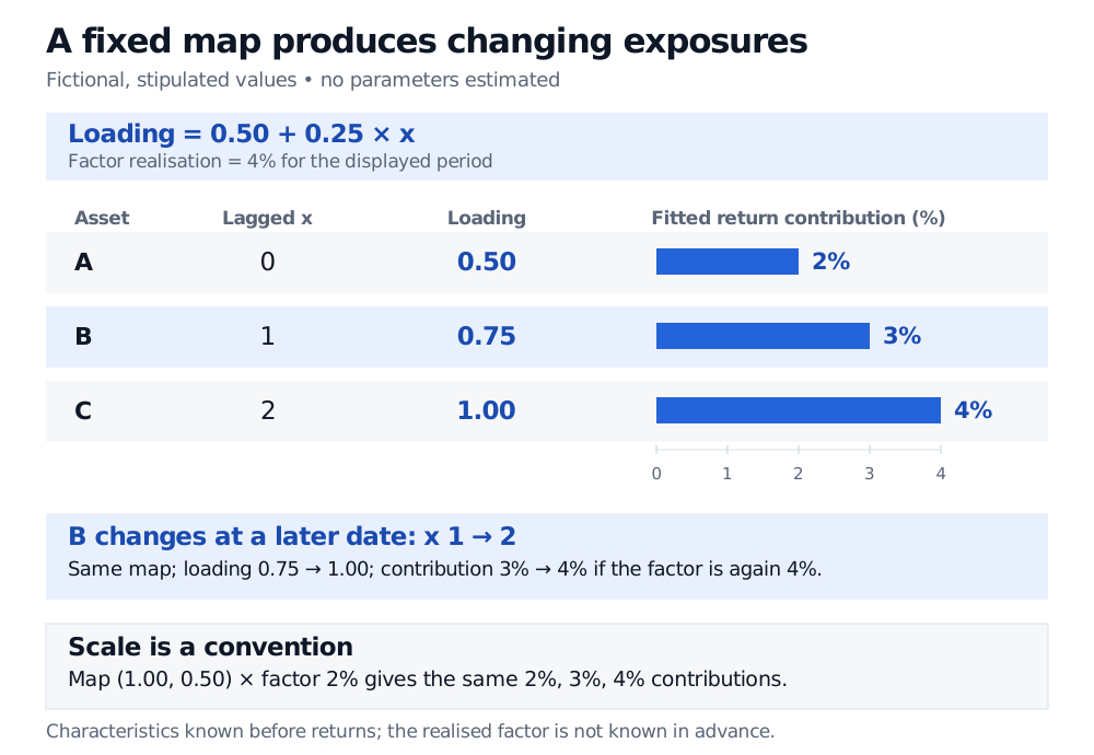
At a later date, suppose B's observable characteristic becomes 2. Its loading becomes 1.00 under the same map. If the next factor realisation is again 4%, B's fitted contribution becomes 4%. Neither the mapping nor the factor has to change to produce this change in exposure.

Stipulated assets A, B and C have lagged characteristic x values 0, 1 and 2, loadings 0.50, 0.75 and 1.00, and fitted contributions 2%, 3% and 4% at a 4% factor realisation. B changing to x of 2 raises its loading to 1.00. Doubling the map and halving the factor leaves all three contributions unchanged.

Original stipulated example. A fixed characteristic-to-loading map permits dynamic exposures; factor and mapping scales can offset each other.

These are fitted contributions given a factor realisation, not forecasts made before that factor is observed. A conditional expected-return forecast also needs a forecast of the factor and appropriate assumptions about the conditional error mean. Actual returns can differ through

e_{i,t+1}

. The constant characteristic contributes to exposure; it is not a separate return alpha in this specification.

Fitting is a different task

IPCA jointly fits

\Gamma

and the factor histories by least squares. Alternating least squares updates factors holding the map fixed, then the map holding factors fixed. The 2019 econometric draft discusses this procedure in §§3.1–3.2. An iteration stopping does not itself certify a global optimum.

Factor rotation leaves fitted returns unchanged: replacing

\Gamma

with

\Gamma H

and

f

with

H^{-1}f

works for any invertible

H

. In this one-factor example, doubling both mapping coefficients and halving the factor gives

(1.00+0.50x)\times0.02 =(0.50+0.25x)\times0.04.

Normalisation selects coordinates; it cannot make these three rows an identified empirical fit. The draft's §3.3 discusses alternative conventions, including orthonormal mapping columns and ordered, diagonal factor second moments; signs still require a convention.

Consistency additionally needs orthogonality between characteristics and composite errors, sufficient rank, and panel moment and dependence conditions. “Instrumented” therefore does not automatically confer the causal interpretation of a valid instrumental-variables design.

Three questions that call for different models

Question	What is being fitted?
Which common movements reconstruct a return panel with static asset loadings?	Ordinary static PCA factor extraction, including asymptotic principal components.
Which characteristics predict future returns?	A characteristic-based forecasting model; latent common factor histories need not be estimated.
Which latent common movements have exposures governed by characteristics?	IPCA estimates the factor histories and a shared characteristic-to-loading map together.

Useful fit does not establish that a component is a priced economic risk, that characteristics cause returns, or that forecasts survive a new period. Changing the characteristic set, preprocessing or factor count changes the model being evaluated.

PCA and Factor Compression develops the static SVD benchmark and its reconstruction criterion. A public preview is available; the full lesson requires membership.

Sources

Bryan Kelly, Seth Pruitt and Yinan Su, “Instrumented Principal Component Analysis”, December 8, 2019, preliminary and incomplete working-paper version. Introduction, equations 1–3; §2.2, assumptions; §§3.1–3.3, estimation and normalisation. This article uses that version's basic model, not a claim about a final econometric publication.
Seth Pruitt, research page, “Characteristics are Covariances: A Unified Model of Risk and Return,” Journal of Financial Economics 134(3), 2019, 501–524, with Kelly and Su; and the separately listed IPCA econometric working paper. The page distinguishes the asset-pricing application from the methodological development.

The fixed object is the map

Three assets, one stipulated factor

Fitting is a different task

Three questions that call for different models

Sources

Related terms

Asymptotic principal components

Factor rotation

Look-ahead bias