Extract common return histories from a smaller time-domain matrix, and distinguish the exact dual-PCA identity from the assumptions needed for latent-factor recovery.
Asymptotic principal components
Asymptotic principal components (APC) estimate common factor histories from a large panel of asset returns using the leading eigenvectors of a time-domain cross-product matrix. When there are many more assets than observation dates, this avoids decomposing a much larger asset covariance matrix. The practical aim is to extract shared movements for statistical risk modelling or performance analysis without specifying economic factor series in advance.
There are two distinct claims to keep separate: dual PCA is an exact matrix identity; latent-factor recovery is a statistical result with assumptions.
Which matrix is being decomposed?
Use N asset rows and T date columns in the return panel R. For covariance-based extraction, demean each asset over time. Define the time Gram matrix
G=NR⊤R,G∈RT×T.
Choose K no larger than the panel rank. Take its K leading unit-length eigenvectors as the columns of VK. A convenient factor normalisation and loading estimate are
F=TVK,TF⊤F=IK,B=TRF.
Here F is T×K: each column is a factor history. B is N×K: each row contains an asset's loadings. Then BF⊤=RVKVK⊤ is the retained PCA fit.
The singular value decomposition makes the duality precise. If R=UDV⊤, then
G=NVD2V⊤,S=T−1RR⊤=T−1UD2U⊤.
The nonzero modes correspond through the same singular values. For a positive singular value dj, uj=Rvj/dj. The eigenvalues of G and sample covariance S differ because their divisors differ. A smaller decomposition changes the computational route, not the retained fit. Forming G still requires processing the asset data; its T×T size does not make all computation independent of N.
Preprocessing changes the question. The original Connor–Korajczyk performance-measurement construction uses excess-return levels, allowing the extracted histories to contain risk premia. Time-demeaning instead isolates variation around each asset's sample mean. State which panel is being analysed; the two should not be silently interchanged.
Four assets, three dates, one pattern
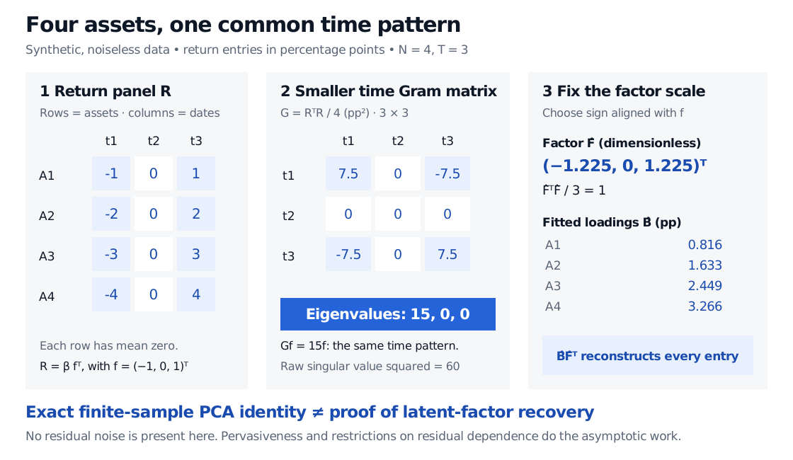
Consider fictional demeaned returns in percentage points:
R=−1−2−3−400001234=βf⊤,β=1234,f=−101.
Since β⊤β=30 and f⊤f=2,
G=7.50−7.5000−7.507.5
has eigenvalues 15,0,0. Its leading unit eigenvector is f/2, choosing the sign aligned with f. Thus
F=23f,B=32β,BF⊤=R.
The raw nonzero singular value squared is 60. Dividing by N=4 gives the time-Gram eigenvalue 15; dividing by T−1=2 gives the asset sample-covariance eigenvalue 30. These values are in squared percentage-point units: compatible descriptions of the same rank-one data.
Noiseless synthetic return panel with four assets and three dates. The time Gram matrix has eigenvalues 15, 0, 0; normalised factor values approximately minus 1.225, zero and 1.225, with loadings 0.816, 1.633, 2.449 and 3.266, reconstruct every return.
Original noiseless example. The smaller matrix identifies the common time direction exactly; the normalisation reallocates scale between factor and loadings. Displayed factor and loading values are rounded.
This calculation contains no residual noise and no limit argument. It verifies the algebra, not an asymptotic theorem.
What earns the word “asymptotic”?
Write the latent model in this article's orientation as
R=BF⊤+E.
Connor and Korajczyk's large-N argument needs pervasive common factors, weak enough cross-asset residual dependence, and moment and time-series restrictions. Pervasiveness means a factor retains non-negligible exposure across the expanding universe; bounded eigenvalues of the idiosyncratic-risk covariance prevent residual dependence from becoming another pervasive source. Approximate factor structure permits some residual correlations.
For the original excess-return panel, a central step is that residual cross-products approach a scalar multiple of the time identity, while factor–residual cross-products vanish. Adding a scalar identity shifts eigenvalues without changing eigenvectors. That mechanism explains why a large cross-section can reveal the factor span. See their §4, especially Theorem 6.
If the panel is time-demeaned, the corresponding residual limit is σ2MT, where MT=IT−11⊤/T. This acts as a scalar identity within the mean-zero time subspace, which is the relevant space for centred PCA. Demeaning also limits rank to at most T−1.
The original unweighted estimator allows bounded differences in idiosyncratic variance across assets. Its restrictions over time are stronger: the cross-sectional average idiosyncratic variance must be time invariant. A date-specific residual-variance surge can distort the time directions instead of acting as a scalar shift. Missing observations also require an explicit extension beyond the balanced-panel calculation. These distinctions are set out in Chen, Connor and Korajczyk, §1.1.
Consequently, large N alone does not guarantee true factors for arbitrary T, weak signals or noisy panels. The realised factor histories must span the required dimensions; subsequent estimation of risk premia or performance parameters also needs adequate time-series information.
A recovered span still needs interpretation
For any invertible H,
BF⊤=(BH−⊤)(FH)⊤.
Factors and loadings therefore need an identification convention. Unit mean-square normalisation fixes scale but still permits orthogonal rotations. PCA with distinct retained eigenvalues selects axes up to sign; factor rotation and sign choices determine the coordinates used to describe the span. In the example, flipping both F and B leaves every fitted return unchanged. With repeated leading eigenvalues, individual eigenvectors are not unique even after ordering them.
An extracted component is consequently not automatically “growth”, a priced risk factor or a profitable trading signal. Examine loadings, residual structure and stability before assigning an economic name.
PCA and Factor Compression develops the SVD, covariance connection and reconstruction-error criterion. It offers a public preview; the full lesson requires membership.
Zhuo Chen, Gregory Connor and Robert A. Korajczyk (2018), “A Performance Comparison of Large-n Factor Estimators”, Review of Asset Pricing Studies 8(1), 153–182. §§1–1.2 distinguish the basic estimator, its heteroskedasticity restrictions and weighted extensions.
Gilbert Strang, Lecture 6: Singular Value Decomposition (SVD), MIT OpenCourseWare, Spring 2018, Summary: shared nonzero eigenvalues of the two cross-product matrices and the mapping between their eigenvectors.