How the candidate functions and preferences built into a learner determine what it predicts beyond its training observations.
Hypothesis space and inductive bias
A hypothesis space is the set of candidate prediction functions a learner can choose from. Inductive bias is the restriction or preference that guides its predictions beyond what agreement with the training observations alone determines. For a quant forecasting returns, choosing linear effects, smooth responses or a particular training procedure helps decide how a fitted relationship extends to market conditions it has not seen.
Mitchell’s original account distinguishes limits on what a learner can represent from preferences in how it searches among representable alternatives. Both matter: making a model class more expressive does not remove the need to choose within it. Mitchell, §§1–4
Two observations do not choose a curve
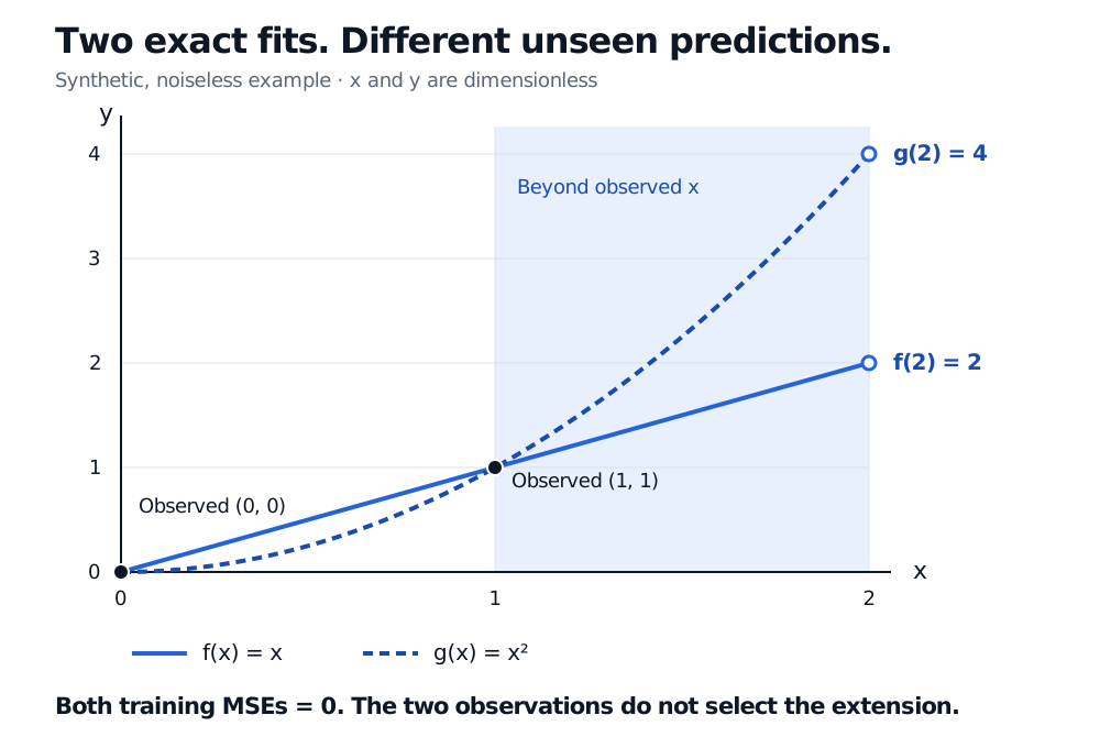
Consider a synthetic, noiseless regression dataset with dimensionless observations (0,0) and (1,1). Two candidates are
f(x)=x,g(x)=x2.
Both predict the observed responses exactly, so both have training mean squared error zero. Yet at the unseen input x=2,
f(2)=2,g(2)=4.
Synthetic observations at (0, 0) and (1, 1) lie on both f(x) = x and g(x) = x squared. Both training mean squared errors are zero; at unseen x = 2, f predicts 2 and g predicts 4.
Original synthetic example. Exact agreement at observed inputs leaves different extrapolations possible; neither curve is labelled as the true relationship.
The ambiguity extends beyond these two candidates. Every member of the family
hc(x)=x+cx(x−1),c∈R,
fits the same observations, because the added term vanishes at both observed inputs. At 2 it gives 2+2c. Thus perfect training fit permits any real prediction there. This is an identification problem in this example, even before introducing measurement noise or a small-sample estimation error.
Restricting the hypothesis space to affine functions a+bx selects a=0,b=1. Allowing quadratics restores the ambiguity. Choosing the straight line because it has lower degree supplies a preference; the two responses did not prove that the unknown relationship is linear. Here x=2 also lies beyond the observed input range, so the disagreement is explicitly about extrapolation.
Where the preference enters
These mechanisms can interact, but describe different modelling decisions:
Decision
What it changes
Example
Hypothesis restriction
Which functions are admissible
Permit affine functions only.
Representation or architecture
How inputs and functions are expressed; sometimes also which functions are possible
Which functions or parameters the stated fitting objective favours
An L2 penalty charges for coefficient magnitude in a specified coordinate system.
Implicit optimisation bias
Which solutions a training procedure approaches without adding that penalty
Initialisation and update rules can select among fits with the same training loss.
A penalty on coefficients depends on their representation and units. “Small coefficients” therefore needs a specified basis and scaling; it does not automatically mean a smooth function. The MAP-estimation lesson derives one precise connection: Gaussian priors on regression coefficients yield a ridge penalty under Gaussian observation noise. The public preview is open; the full lesson requires membership.
A concrete implicit-bias result comes from Soudry and coauthors. For unregularised logistic regression with homogeneous linear predictors on linearly separable data, gradient descent with an appropriately bounded constant step size approaches the direction of the Euclidean maximum-margin separator. The coefficient norm itself diverges. This is a conditional result about a particular loss, model and training procedure, not a guarantee for arbitrary neural networks or optimisers. Soudry et al., introduction and §2
Why some structure has to earn our trust
The no free lunch theorem concerns specified averages over problems, rather than equality on each dataset. One simple classification setting makes the distinction clear: take a finite input domain, binary target labels, a uniform distribution over all deterministic target functions, fixed observed inputs and their noiseless labels, and zero–one loss on an unobserved input. Conditional on the observations, either unseen label is equally likely. Any learner predicting a binary label without further target information has expected error one half there. Changing the distribution over targets can break that equality. Wolpert, §4
The ugly duckling theorem illustrates a related symmetry in similarity: on a finite distinguishable universe, treating every subset predicate equally makes every distinct pair share the same number of true predicates. Choosing features or weights breaks that symmetry. It is a counting result about similarity, not a prediction-error theorem. Watanabe, §1.7
For financial research, a useful bias needs a reason to match the task: for example, an economically motivated response shape or a representation suited to the forecast horizon. Evaluate that choice on held-out periods with the information available at each forecast time. Neither a more flexible hypothesis space nor a stronger simplicity preference guarantees better generalisation, especially when market relationships change.
Finally, inductive bias names a learning assumption or preference. Statistical prediction bias, used in the bias–variance tradeoff, measures a systematic prediction discrepancy under a specified repeated-sampling model. Social bias concerns unfair or prejudicial patterns affecting people. These meanings can interact in an application, but they are not interchangeable.