Why equal average performance over all target functions does not imply that prediction methods are equally useful on structured financial data.
No free lunch theorem
The no free lunch theorem is a family of results showing that algorithms have equal performance under specified ways of averaging over problems. A basic supervised-learning version averages uniformly over all binary target functions and measures errors only at inputs absent from training. For quant research, its consequence is that a universal claim of predictive superiority needs assumptions about which financial relationships are plausible. It does not establish equality on actual market data. Wolpert, introduction and §4
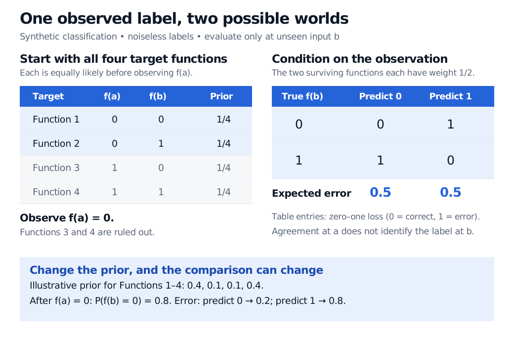
A complete example with four possible worlds
Take two distinct inputs, a and b, with noiseless labels in {0,1}. Fix the training input at a, independently of the target function. Before seeing its label, give each possible target probability 1/4:
Target
Label at a
Label at b
Function 1
0
0
Function 2
0
1
Function 3
1
0
Function 4
1
1
Now observe f(a)=0. Only Functions 1 and 2 remain compatible. Conditional on this observation, each has probability 1/2.
A learner must predict a binary label at the unseen input b. Predicting 0 is correct for Function 1 and wrong for Function 2; predicting 1 reverses those outcomes. Under zero–one loss, an error costs 1 and a correct prediction costs 0. Either prediction therefore has expected loss
21×0+21×1=21.
Four binary target functions start with probability 1/4 each. Observing f(a) = 0 leaves output pairs (0, 0) and (0, 1), each with probability 1/2. Either prediction at b has expected error 0.5. An illustrative prior of 0.4, 0.1, 0.1, 0.4 changes those conditional probabilities to 0.8 and 0.2.
Original finite classification example. Equal weighting leaves the unseen label balanced; the separate illustrative prior favours matching labels and breaks the tie.
The statement concerns an average, not identical outcomes: on Function 1, the prediction 0 wins outright. Nor is randomisation an escape. If the learner independently predicts 1 with probability q, its expected error is q/2+(1−q)/2=1/2.
The same counting argument works on a larger finite input domain. With a uniform prior over every binary target function and fixed observed inputs with noiseless labels, each compatible target can be paired with another that differs only at the particular unseen input being tested. The pair has equal probability and opposite labels there. Any binary prediction is wrong on exactly one member.
The test criterion matters. Here “unseen” means an input value absent from training, not merely a different database row. A fresh draw can repeat a training input on a finite domain. Loss averaged over the entire domain can include such observed inputs, where a memorising learner already knows the noiseless label. That is a different criterion from the off-training-set error used here. Wolpert, §§4–5
What changes when a preference has information?
Keep the same four targets, but assign them probabilities 0.4, 0.1, 0.1 and 0.4 respectively. This is an invented prior that favours equal labels at the two inputs; it is not a model of market data.
After observing f(a)=0, the probabilities of Functions 1 and 2 become 0.8 and 0.2. Predicting 0 at b now has expected error 0.2; predicting 1 has expected error 0.8. Repeating the observed label also beats flipping it before conditioning: averaging directly over all four targets gives the same 0.2 versus 0.8 errors.
An inductive bias is useful when its preference aligns with the task. Merely saying “the prior is nonuniform” does not identify a winning rule: its actual weights matter. The constructed comparison shows how an assumption can help, rather than proving that any particular financial assumption is true.
For example, expecting nearby economic conditions to produce related responses favours some target functions over others. Whether a chosen representation captures that structure remains an empirical question. A realistic performance comparison specifies the forecast horizon, available information, loss and evaluation periods. The theorem supplies no ranking of linear models, trees or neural networks for such a task.
The optimization theorem is a separate statement
Wolpert and Macready’s finite black-box optimization result concerns sequentially choosing inputs to evaluate an objective. In its basic static form, the search domain and objective-value set are finite, and the average is uniform over all functions between them. Algorithms choose previously unvisited points; performance is assessed after the same number of distinct evaluations using the observed objective values, such as their minimum. Under this setup, the distribution of the observed value sequence is independent of the search algorithm when averaged over all objectives. Wall-clock runtime is outside that comparison. Wolpert and Macready, §§II–III
This compares search trajectories, whereas the classification example compares predictions at a fixed unseen input. Neither result says that two algorithms tie on each problem, that every loss has the binary classification result above, or that structured financial problems inherit the uniform average.
For a complementary result under explicit sampling and hypothesis-class assumptions, the SelfMadeQuant lesson Sample Complexity Bounds derives finite-class uniform convergence and compares empirical risk minimisation with the best function in that class. A public preview is available; the full lesson requires membership.