GraphSAGE learns a reusable neighbourhood aggregation function. Follow a mean-aggregation example, distinguish inductive embeddings from DeepWalk, and check graph information time.
GraphSAGE
GraphSAGE is an inductive graph neural network framework that learns a function for generating a node's embedding from its features and neighbourhood. Its name abbreviates “sample and aggregate”. For a quant modelling firms or accounts as nodes, the practical attraction is producing a representation for a newly observed entity without first fitting a separate embedding vector for that entity. Hamilton, Ying and Leskovec introduced the framework in 2017.
Consider a hypothetical supplier network used to study corporate distress. A firm's own attributes describe it directly; its neighbours' attributes can describe the firms to which it is connected. This is a modelling choice: a supply relationship has a direction, and customers and suppliers need not carry the same information.
A function that transfers to new nodes
At each layer, GraphSAGE summarises neighbours' previous-layer representations and combines that summary with information about the root node. Repeating layers reaches further into the graph. Sampling a bounded number of neighbours at each depth limits the computation, while introducing sampling variability. The framework permits supervised training against a task label or unsupervised representation learning. These choices are described in the original paper, §§3.1–3.3.
The contrast with DeepWalk concerns what is learned. Standard DeepWalk learns a table of node-specific vectors from random-walk contexts. Its online procedure can update that table, but a new node does not receive an embedding merely by passing its attributes through a learned feature-aggregation function. GraphSAGE supplies such a reusable function. See DeepWalk, §§3.3–4.2 and §4.4.1.
Inductive capability does not guarantee generalisation: a new entity still needs usable features and a neighbourhood, with meanings compatible with training. A changed reporting regime or a different kind of edge can change what the representation measures.
Trace one chosen mean-aggregation layer
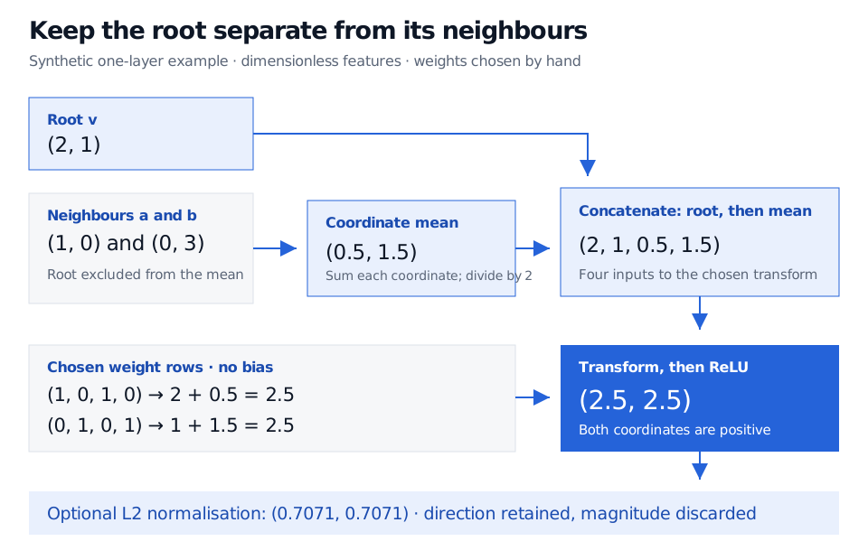
Use a synthetic root feature vector xv=(2,1)⊤ and exactly two neighbours, xa=(1,0)⊤ and xb=(0,3)⊤. All features are dimensionless. This example uses a neighbour mean excluding the root, concatenation, no bias, and a ReLU activation. The weights are chosen by hand.
The neighbour summary and concatenated column vector are
The first output is the root's first coordinate plus the neighbours' mean first coordinate: 2+0.5=2.5. The second is 1+1.5=2.5. ReLU applies max(0,z) to each coordinate, so it leaves both positive values unchanged. The result is a representation, not a distress probability.
Synthetic one-layer GraphSAGE calculation: neighbour features (1, 0) and (0, 3) average to (0.5, 1.5). Concatenate root (2, 1) to form (2, 1, 0.5, 1.5). The chosen weight rows produce (2.5, 2.5); optional L2 normalisation gives approximately (0.7071, 0.7071).
Original synthetic calculation, all features dimensionless. The root is excluded from the neighbour mean and retained separately. Parameters are stipulated, with no fitted model or performance claim.
If this layer additionally applies unit-length normalisation, its output becomes
∥hv∥2hv=(1/21/2)≈(0.70710.7071).
This discards the vector's magnitude. Normalisation requires a convention for a zero vector; the displayed nonzero example avoids that case.
Specify the variant. The paper's Algorithm 1 includes concatenation and normalisation, while its convolutional variant combines the root with neighbours in a joint mean. Implementations also differ: PyTorch Geometric's documented SAGEConv operator adds separately transformed root and neighbour-mean terms and defaults to no output normalisation. Splitting the columns of a concatenation weight matrix gives that same linear combination when the other settings agree. Neither literal concatenation nor unit normalisation is a universal requirement of everything called GraphSAGE.
INTERACTIVE EXPLORER
Typed graph-message aggregation
Update scalar node features along a small directed graph.
A graph can leak tomorrow's information
For the hypothetical supplier model, define the graph as it was knowable at the decision time. A relationship announced next month cannot enter today's neighbourhood merely because a current database records it. Apply the same rule to node features: revised accounts, later distress flags and full-history scaling can introduce look-ahead bias. Even an unlabelled future node can reveal future structure through its edges.
Sampling must draw from this eligible graph, rather than sampling first and filtering only the root's attributes. For evaluation, keep training labels available by the fit cutoff and reproduce the intended schedule for fitting, graph updates and inference. A random node split alone cannot establish a valid historical forecasting experiment.
The mean also compresses information: different neighbour sets can have the same coordinate averages. In this example, swapping the two neighbours changes nothing, but replacing them with two copies of their mean also changes nothing. Whether that loss matters depends on the task; aggregation does not establish that connected firms share the same risk.