Gradient saliency measures local input sensitivity. Separate it from finite attribution, account for units and probability saturation, and understand what SmoothGrad averages.
Gradient saliency and SmoothGrad
Gradient saliency measures how a selected model output changes under tiny changes to each input, at one particular observation. SmoothGrad averages such sensitivity maps over noisy versions of that observation. For a quant inspecting a return forecaster or credit classifier, these methods can flag inputs to investigate: which features would move this model score locally, and how stable is that answer to a specified perturbation?
The result describes the fitted computation. It does not identify an economic cause, a trading signal or an allocation of the entire prediction. This distinction matters even in a one-variable model.
The tangent is not the journey
Let f(x) be the scalar target being explained. The signed saliency for input i is the partial derivative
gi(x)=∂xi∂f(x),f(x+Δx)−f(x)≈i∑gi(x)Δxi.
This approximation is local. It holds near a differentiable point, with the model and other inputs fixed when taking each partial derivative. Simonyan, Vedaldi and Zisserman, §3 motivate image saliency through this first-order approximation. The same calculus applies to differentiable financial predictors.
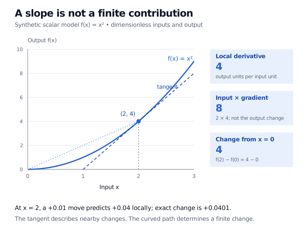
Consider the synthetic, dimensionless score f(x)=x2 at x=2. Its derivative is f′(2)=4. A move of +0.01 therefore predicts a score change of approximately 4(0.01)=0.04; exact revaluation gives 2.012−22=0.0401.
Three quantities that are easily confused now separate:
Quantity
Calculation
Meaning
Local gradient
f′(2)=4
Slope at the current input
Gradient × input
2f′(2)=8
A different attribution heuristic
Change from reference zero
f(2)−f(0)=4
Finite output difference
Multiplying by the input does not turn the tangent into the accumulated change. In this curved model, the slope varies between zero and two. Integrated gradients addresses a different question by integrating derivatives along a chosen reference-to-input path; the reference still needs a defensible meaning.
For the synthetic dimensionless model f(x)=x squared, the point is (2,4), the local slope is 4, gradient times input is 8, and the output change from reference zero is 4. A tangent at x=2 differs from the curved path.
Original synthetic quadratic example. Local sensitivity, gradient × input and a finite reference-relative change are different quantities, even when two happen to share the number four.
At x=0, the gradient of this same model is zero, yet moving to x=0.1 raises the output by 0.01. Zero saliency means no first-order sensitivity at that point; curvature can still matter. At a nondifferentiable activation boundary, software uses a specified derivative convention, so the mathematical qualification also matters.
The owned Partial Derivatives lesson develops gradients, scenario changes and the distinction between a partial sensitivity and realised change (public preview; full lesson requires membership).
Choose the output and its units first
A neural network can return many numbers. Explain one declared target: a return forecast for a stated horizon, a class logit, a class probability, or a loss. The derivative of the loss answers a different question from the derivative of the prediction. Computing input saliency keeps learned weights fixed; it is not the training update to those weights.
Output transformations can change the apparent sensitivity substantially. For a binary classifier with logit z and probability p=1/(1+e−z),
∂xi∂p=p(1−p)∂xi∂z.
In a synthetic model with z=x, at x=8 the logit derivative is one, but p≈0.999665 and the probability derivative is only 0.00033524. The probability is saturated near one. A small probability gradient does not demonstrate that the feature played little part in reaching that prediction. Conversely, a logit gradient is in logit units, not probability points. In multiclass softmax models, a class probability also depends on competing class scores.
Input units matter just as much. Suppose a synthetic score is y=2r, where r is a decimal return. If the identical input is recorded in percentage points, q=100r, the same score is y=0.02q. The raw gradient changes from two to 0.02. A one-percentage-point scenario gives the same score change either way: 2(0.01)=0.02(1)=0.02.
Record scaling and preprocessing with the map. For standardised features, the gradient is per standardised input unit unless the derivative is propagated back through the scaling. Comparing raw gradient magnitudes across dollars, ratios and percentage points is not a unit-free feature ranking.
What does adding noise average away?
Derivatives can change sharply between neighbouring inputs, particularly across activation boundaries. Smilkov et al., §2.2 propose averaging sensitivity maps from Gaussian-perturbed inputs. For signed-gradient SmoothGrad, one common specification is
gσ(x)=N1k=1∑N∇f(x+ϵk),ϵk∼N(0,σ2I)
with independent noise draws. It estimates an average gradient over the chosen neighbourhood, rather than the derivative at the original point. Increasing N reduces sampling variability around that average; changing σ changes the neighbourhood and the quantity being estimated. Feature-specific noise scales or a covariance structure can be appropriate, but must be declared.
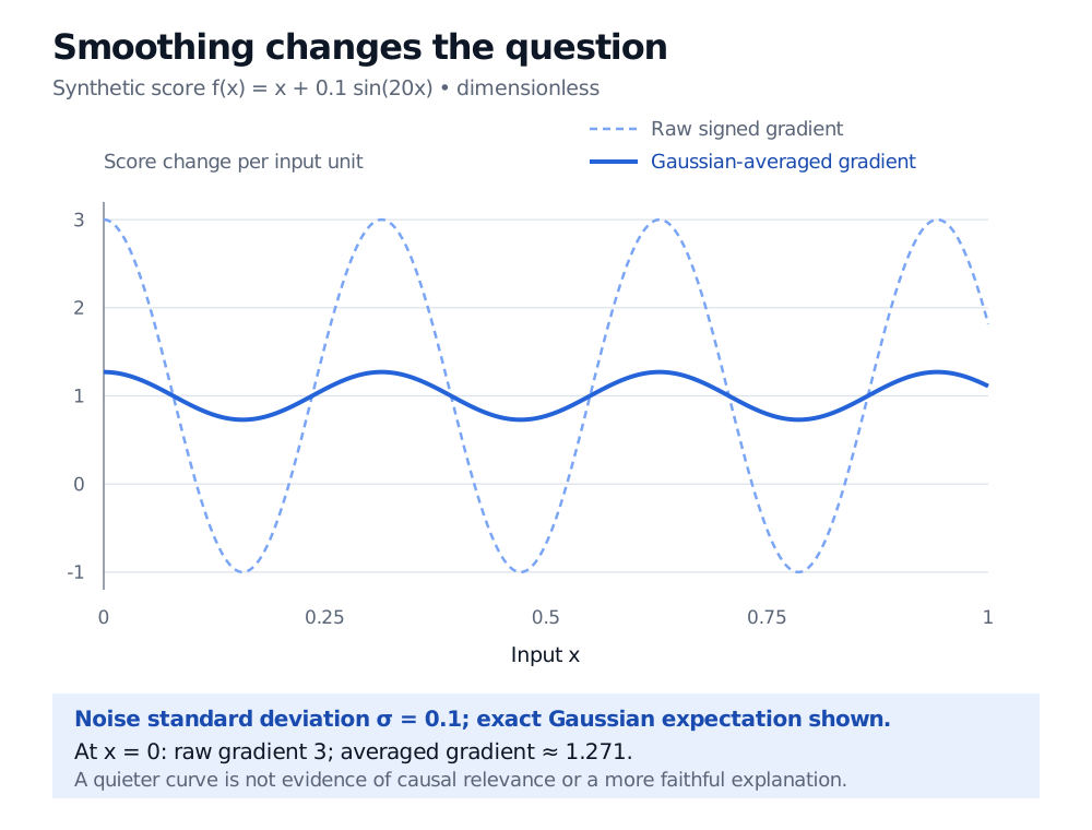
The next figure isolates the averaging mathematically. For the synthetic score f(x)=x+0.1sin(20x), the raw derivative is 1+2cos(20x). Averaging it over Gaussian noise with standard deviation 0.1 gives the exact expectation 1+2e−2cos(20x). At zero, the original slope is three and the averaged slope is approximately 1.271. This is a deliberately constructed illustration, not a fitted financial model or an empirical claim of improved explanations.
A synthetic score x plus 0.1 sin(20x) has an oscillating signed derivative between minus 1 and 3. Gaussian averaging with standard deviation 0.1 reduces the oscillation: at x=0 the raw derivative is 3 and the exact averaged derivative is about 1.271.
Original synthetic gradient comparison. The solid line shows the exact Gaussian expectation, not a finite Monte Carlo sample; the dashed line shows the derivative at each unperturbed input. All quantities are dimensionless.
Taking absolute values before averaging discards cancellation between positive and negative slopes. Taking the absolute value after averaging preserves that cancellation before hiding direction. Averaging squared gradients is another construction again. Captum's Saliency documentation returns absolute gradients by default; its NoiseTunnel documentation distinguishes mean attributions, mean squared attributions and attribution variance. State the actual combination used rather than reporting only “SmoothGrad”.
For financial tabular data, independent Gaussian perturbations may create impossible leverage values or break relationships between prices, returns and accounting ratios. Clipping invalid draws changes the effective neighbourhood. Smoother pictures cannot resolve those modelling choices, and image-based findings do not automatically validate a perturbation scheme for market data.
Test the explanation against the model
A useful diagnostic should respond to what the fitted predictor learned. Adebayo et al. test this by randomising learned parameters and by retraining on permuted labels. They show that some visually convincing saliency methods can remain insensitive to such changes. Their experiments do not imply that every gradient method fails; ordinary gradients passed their reported sanity checks.
For a financial model review, retain signed values and an unnormalised scale alongside any heatmap. Compare gradients with small, valid finite perturbations of the declared target. Examine dependence on the noise scale and preprocessing, and compare explanations across model versions and dated observations. Randomisation tests probe dependence on learned parameters or labels; passing them is useful evidence, not proof of a complete explanation. Time-series label permutations also destroy temporal structure, so interpret that experiment according to its diagnostic purpose.
Use the map to guide an investigation: a large sensitivity to a suspicious input warrants checking its construction and availability. It does not establish causal inference, forecast accuracy or reliability outside the observed neighbourhood. The broader XAI framework helps choose which of those questions actually needs answering.