Gamma and Tweedie regression are generalised linear models for outcomes whose variability grows with their conditional mean. Gamma regression models strictly positive continuous responses, such as claim severity conditional on a claim occurring. Tweedie regression with power between one and two can model aggregate claim cost, including periods with no claims. Choosing between them changes which outcomes the model can explain, even when both use the same positive mean prediction.
Start with the response, then choose the link
For a response , predictors and unit observation weights, write
Here is dispersion. The log link makes positive and gives multiplicative effects: a one-unit increase in predictor multiplies the mean by , holding everything else fixed. It links the mean, rather than fitting a regression to observed . The log link is a choice; it is not the canonical link for Gamma regression. Software defaults differ: statsmodels' Gamma documentation specifies an inverse default and explicitly permits log.
| Response family | Power | Possible realised responses | Typical cost target |
|---|---|---|---|
| Gamma distribution | Strictly positive continuous values | Severity among positive claims | |
| Compound Poisson–Gamma Tweedie | Zero plus positive continuous values | Total cost including no-claim observations |
Tweedie is a wider family; this article focuses on the cost-modelling range , with Gamma at . A positive fitted mean does not prevent the first model from rejecting exact zeros or the second from assigning them probability. Neither row is a model for negative net P&L; the second is not a count-only distribution. R's official Tweedie documentation describes this support distinction.
The zero comes from a random number of costs
At fixed predictors, a Tweedie response in this range has a compound Poisson representation:
The severities are independent and identically distributed, independent of ; is scale, not rate. An empty sum is zero. Because each severity is positive, exactly when , giving . Conditional on a positive count, the sum is continuous and positive. The SAS/STAT derivation connects this construction to the mean–dispersion parameters.
This differs from arbitrarily adding a separate zero-inflation probability: the Tweedie zero probability is tied to its distributional parameters. A dataset's zero frequency and positive-cost shape therefore both matter when checking the model. A Gamma severity regression alone also leaves claim frequency unresolved.
One mean, two variance specifications
Consider a fictional cost model at one unit of exposure, with mean currency units. Specify numerical dispersion separately in each family. Then
Both variances have units of currency squared. These stipulated values illustrate the variance powers, not a model ranking. If the response has currency units, has units of currency to the power : dimensionless for Gamma and square-root currency for . Equal numerical dispersions are not equal physical quantities across these powers. Each model's dispersion must be estimated under its own specification.
As an independent check, the Gamma example has shape and scale , yielding variance . These are the usual shape–scale Gamma moments. The Tweedie example can instead be built with , and . Its random-sum variance is , agreeing with .
Exposure changes the total, and needs a variance convention
Let denote exposure relative to a chosen unit, and the expected cost per unit exposure. For an aggregate response , a proportional mean model is
The known is an offset, whose coefficient is fixed at one. At the same predictors, gives expected totals of at exposure one and at exposure two. This assumes the modelled cost rate persists across the longer exposure. The official GLM documentation states how log exposure enters the predictor.
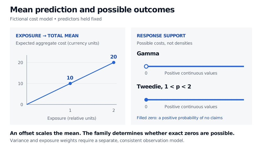
Original specified mean model and support schematic. The support lines show possible responses, not probability densities or the size of the zero mass.
The offset alone says nothing about how variance aggregates. Under independent, homogeneous additive exposure increments with unit-exposure variance ,
Thus a rate response has mean and inverse-exposure dispersion. An implementation using the convention represents this with variance weight , rather than merely repeating the row. Equivalently, for an aggregate response with mean , effective dispersion is . Holding aggregate dispersion constant while adding an offset specifies a different variance model. Smyth and Jørgensen (2002), §2, formulate costs per unit risk with exposure in the variance denominator. This convention requires its independence and homogeneity assumptions; it is not a universal law for pooled portfolios with shared shocks or changing risk mix.
For the underlying GLM construction, The Exponential Family and Generalized Linear Models develops canonical-link Bernoulli and Gaussian examples. A public preview is available; the full lesson requires membership. The log-linked Gamma model here illustrates the broader choice of a noncanonical link.
Sources
- Smyth and Jørgensen (2002), Fitting Tweedie's Compound Poisson Model to Insurance Claims Data: Dispersion Modelling, §§1–2.
- R mgcv: GAM Tweedie families, Arguments and Details.
- SAS/STAT 13.2: Tweedie Distribution for Generalized Linear Models, used for distributional identities, not current software defaults.
- statsmodels: Gamma family and GLM offsets, exposure and weights.
- NIST/SEMATECH: Gamma Distribution, density and common statistics.