A factorisation machine shares latent feature vectors across interaction coefficients. Follow a pairwise score of 6 and the fast evaluation identity, with sparse-data and financial-timing limits.
Factorisation machine
A factorisation machine (FM) predicts from features using interaction coefficients built from shared latent vectors. For a quant working with sparse security, sector and event indicators, it offers a way to model combinations without fitting every pair independently. Whether those combinations improve a financial forecast remains an empirical question.
Here w0 is an intercept, wi a linear coefficient, and each feature has a length-k latent vector. The dot product gives the pair coefficient. The index condition i<j counts each distinct pair once and excludes self-interactions. This is a second-order model: three-way and higher interactions require an explicit extension. Rendle's original paper, §III, defines this distinction.
Synthetic calculation. Set x1=2, x2=3, v1=(1,2) and v2=(3,−1). These are stipulated dimensionless values, not fitted financial data. Then
⟨v1,v2⟩=1(3)+2(−1)=1,I(x)=1(2)(3)=6.
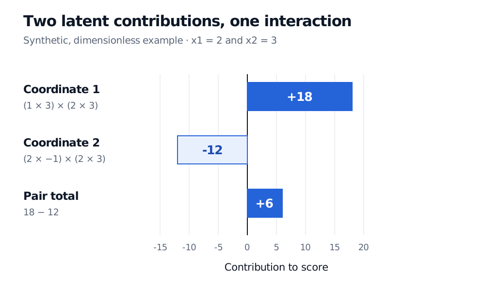
The interaction adds 6 to the intercept-plus-linear score; it is the entire prediction only if those other terms are zero. Its two latent-coordinate contributions are 18 and −12.
Synthetic dimensionless FM: feature values 2 and 3 with latent vectors (1, 2) and (3, −1) give coordinate contributions +18 and −12, for a pairwise interaction of +6.
Original synthetic example. Opposing latent-coordinate contributions can partly cancel; the pair coefficient is the dot product, not either coordinate alone.
Factorisation does not require positive interactions. In the same synthetic setup, replacing v2 by (−1,−2) makes the coefficient −5 and the interaction −30. Nor does “latent factor” identify an economic risk premium: the coordinates are model parameters, without an automatic financial interpretation.
Shared information, with a fast calculation
A feature vector is reused in every pair containing that feature. Observations involving one pair therefore affect other pair estimates through the shared parameters. This can help when individual pairs rarely co-occur; it does not supply reliable estimates for a completely unseen identity with no informative attributes. The sharing mechanism is developed in Rendle (2010), §III.A.3.
The interaction can be evaluated without enumerating every pair:
I(x)=21f=1∑k(i=1∑pvifxi)2−i=1∑pvif2xi2.
In the example, the weighted feature values in coordinate 1 are 2 and 9. Their squared sum is 121; their sum of squares is 85. Coordinate 2 gives 4 and −3, with corresponding values 1 and 25. Hence
I(x)=21[(121−85)+(1−25)]=6.
Subtracting the squares removes the self-products; halving removes double counting. With m nonzero features, this computation takes O(km) arithmetic rather than O(km2) for direct pair enumeration. See Rendle's Lemma 3.1.
What the data must mean
Imagine a hypothetical next-period return model whose features include a security identity, sector, an earnings-event indicator and a liquidity measure. Most identity columns are zero in each row. An FM could share security–event and sector–liquidity structure, but this is a proposed modelling use, not evidence of predictive performance.
The fitted objective must match the target. A return forecast, binary outcome and recommendation ranking need different losses. Latent dimension and regularisation control flexibility; neither sparsity nor factorisation prevents overfitting. The author's libFM manual, §§3.1–3.3 separates model dimensions, prediction tasks and learning settings.
For financial evaluation, build point-in-time features: use the sector classification, event information and liquidity observations available at the decision. Fit preprocessing and tune settings on permitted training and validation periods, then assess a later test. The Time-Ordered Train, Validation and Test Design lesson develops that schedule; its preview is public and the full lesson requires membership.
A separate application is ranking research reports for users from readership logs. Here unread is not automatically disliked: a report may never have been shown. Turning every missing user–report pair into a negative label changes the learning problem. Rendle and co-authors' BPR paper, §3 explains this ambiguity for implicit feedback. A zero in a feature vector and an unobserved target are different things.
Sources
Steffen Rendle, Factorization Machines, ICDM 2010, pp. 995–1000, §III.A–D: second-order model, parameter sharing, efficient evaluation and higher-order extension. Original paper, accessible copy; the author's libFM bibliography identifies it as the introductory paper.
Steffen Rendle, libFM 1.4.2 Manual, 14 September 2014, §§3.1–3.3: dimensions, tasks, regularisation and learning settings. This is a versioned implementation reference.
Steffen Rendle, Christoph Freudenthaler, Zeno Gantner and Lars Schmidt-Thieme, BPR: Bayesian Personalized Ranking from Implicit Feedback, UAI 2009, §3: unobserved pairs can mix negative preferences and missing observations; arXiv copy posted in 2012.