Use multiscale covering numbers to bound process suprema, evaluate a finite entropy-integral proxy, and distinguish Gaussian and empirical Rademacher conventions.
Dudley entropy integral
The Dudley entropy integral adds up the geometric complexity of a model class across approximation scales to bound the expected maximum of a random process. For a quant researcher comparing many predictors, it helps quantify how much apparent performance can arise from searching a rich class: nearby predictors should not be counted as independent opportunities to fit noise.
The geometry enters through the covering number, N(T,d,ε): the smallest number of radius-ε balls, with centres in T, needed to cover an index set T under distance d. Here and below, log is the natural logarithm. The entropy is logN; Dudley integrates its square root.
The distance must describe the noise
Let (Xt)t∈T be a centred, separable process: E[Xt]=0, and a countable subset suffices to determine its supremum almost surely. Suppose d is a pseudometric satisfying the increment bound
E[eλ(Xt−Xs)]≤exp(2λ2d(s,t)2)for every s,t∈T,λ∈R.
Thus differences are sub-Gaussian at scale d(s,t). A pseudometric permits distinct indices to have zero distance.
Write D=sups,t∈Td(s,t)<∞. For totally bounded (T,d), one standard form is
E[t∈TsupXt]≤C∫0DlogN(T,d,ε)dε,
where C is a positive universal numerical constant, independent of the process and T. This states a bound up to a constant, not an equality or a sharp numerical estimate. Beyond D, one ball suffices. These conventions follow Duchi’s sub-Gaussian process notes, slides 4 and 7–10.
For a centred Gaussian process, the classical choice is its canonical pseudometric,
d(s,t)=E[(Xs−Xt)2].
For a general process, this standard deviation alone need not satisfy the displayed exponential bound. The chosen distance must control the increments’ tails. Also, the displayed supremum has no absolute value. A bound for E[supt∣Xt∣] must account for an anchor value, or otherwise control the absolute level. These distinctions are developed in Tropp’s notes, §§12.1–12.4, and Duchi’s slide 12.
Why integrate over every scale?
A single cover replaces every model by one representative. Chaining instead uses a succession of finer covers and writes each process value as a coarse value plus successive refinements. Fine refinements are numerous, but their increments are small. Summing the costs across scales produces the integral. Tropp, §§12.2–12.3, develops this argument.
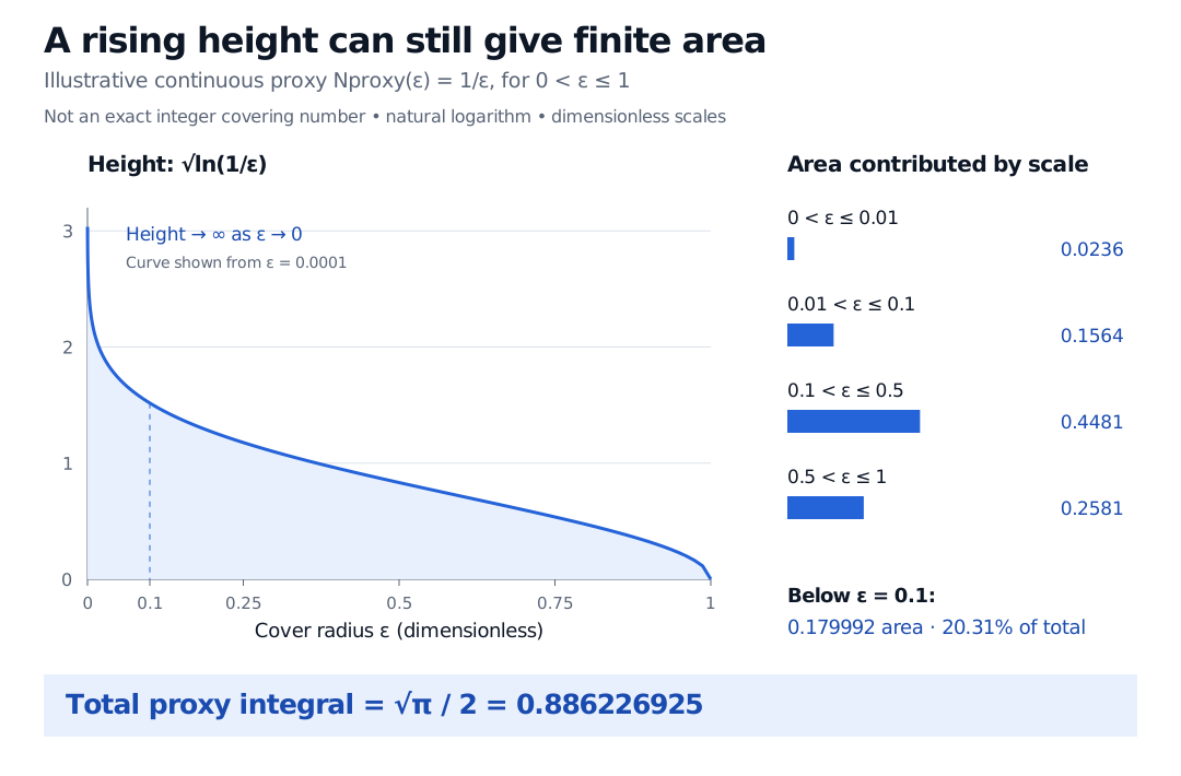
To see the accumulation without hiding it inside a theorem, use the continuous illustrative proxy
Nproxy(ε)=ε1,0<ε≤1.
It resembles the inverse-radius growth of covers of a one-dimensional interval, but is not its exact integer covering number. It is neither an asserted upper bound under our covering convention nor an actual process specification. The following number therefore illustrates the integral; it is not a computed expected maximum.
Iproxy=∫01log(1/ε)dε.
Put u=log(1/ε), so ε=e−u2 and dε=−2ue−u2du. Then integration by parts gives
The boundary term ue−u2 vanishes at both endpoints. Although the original integrand tends to infinity at zero, its area is finite. Scales below 0.1 contribute about 0.179992, or 20.31% of the total. A tall integrand over a narrow range need not dominate the integral.
Continuous illustrative covering proxy Nproxy equals one over epsilon, not an exact cover. Its entropy integral is 0.886227; scales below epsilon 0.1 contribute 0.179992, or 20.31 percent.
Original proxy calculation, not empirical data or an exact covering number. The curve is shown from epsilon 0.0001; the reported areas include the limiting interval down to zero.
For the limiting-area idea, Improper Integrals covers integrable endpoint singularities; its full teaching requires membership, with a public preview.
From Gaussian suprema to empirical Rademacher complexity
The classical Gaussian bound and the empirical learning bound share a chaining argument; their normalisations differ. Fix observations x1,…,xn and a function class F containing zero, with finite empirical radius R. Define
where the independent signs σi equal +1 and −1 with equal probabilities. For measurable suprema and R>0, a refined Rademacher complexity bound is
Rn(F)≤0<α≤Rinf{4α+n12∫αRlogN(F,dn,ε)dε}.
If R=0, the complexity is zero. This is the normalisation in Srebro and Sridharan’s refined bound, Theorem 2, specialised to a class containing zero. The signed-average process has sub-Gaussian increment metric dn/n: the factor 1/n is essential. Distinct functions agreeing on the sample have zero empirical distance. The inner-product and norm lesson develops the geometry behind such distances; full lesson membership is required, with a public preview.
The cutoff α balances unresolved fine-scale error against covering complexity. If the integral from zero diverges, the untruncated upper bound is inconclusive: divergence does not prove that the process is unbounded. A truncated bound or finer chaining analysis may still help. These limitations appear in Srebro and Sridharan, §2, and Tropp, §§12.5–13.2.
For financial data, this conditional geometric calculation does not itself justify an independent-sample generalisation theorem. Serial dependence, overlapping labels and selection using future information require their own treatment.