Covering number and metric entropy: Definition & Examples

A covering number is the smallest number of representative points needed to approximate every point in a set within a specified distance tolerance. Metric entropy is the logarithm of that number. For a quant modelling an infinite family of return forecasts, this provides a way to count distinguishable prediction patterns at a chosen resolution rather than count parameter values.

State the distance and the covering rules

Let

T

be a nonempty subset of a metric space, with distance

d

, and let

\varepsilon>0

. This article uses closed balls with centres in $T$ . Its covering number is

N(T,d,\varepsilon)=\min\left\{m:\ \exists c_1,\ldots,c_m\in T,\quad \forall t\in T,\ \min_{1\leq j\leq m}d(t,c_j)\leq\varepsilon\right\}.

Set

N=\infty

if no finite cover exists. A set of centres satisfying the distance condition is an $\varepsilon$ -net; it need not have the smallest possible size. Exhibiting ten suitable centres proves only

N\leq10

These are Vershynin's covering conventions. Other authors allow centres outside

T

, or use the strict inequality

d(t,c_j)<\varepsilon

. Keep the convention attached to an exact count.

Two balls really are enough—and necessary

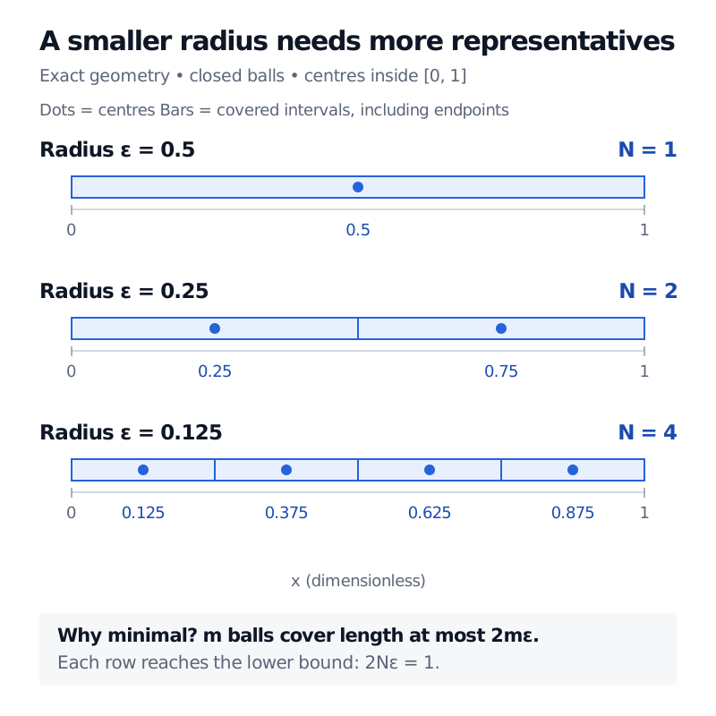
Take $T=[0,1]$ with ordinary absolute distance $d(x,y)=\lvert x-y\rvert$ . All coordinates and radii here are dimensionless. At radius $\varepsilon=0.25$ , the centres $0.25$ and $0.75$ cover respectively $[0,0.5]$ and $[0.5,1]$ . Their union contains every point, including the meeting point $0.5$ .

That proves $N\leq2$ . For the reverse inequality, one radius- $0.25$ ball has length at most $0.5$ inside the interval, so it cannot cover an interval of length $1$ . Therefore

N([0,1],\lvert\cdot\rvert,0.25)=2.

The same argument works at every positive radius. If $m$ balls cover the interval, their union has length at most $2m\varepsilon$ , so $m\geq\lceil1/(2\varepsilon)\rceil$ . Conversely, partition $[0,1]$ into that many equal subintervals and place a centre at each midpoint. Each half-width is at most $\varepsilon$ . Thus

N([0,1],\lvert\cdot\rvert,\varepsilon) =\left\lceil\frac{1}{2\varepsilon}\right\rceil.

Radius $\varepsilon$	One smallest set of centres	Covering number
$0.5$	$0.5$	$1$
$0.25$	$0.25,\ 0.75$	$2$
$0.125$	$0.125,\ 0.375,\ 0.625,\ 0.875$	$4$

Closed-ball covers of the dimensionless interval from 0 to 1: radius 0.5 needs 1 centre at 0.5; radius 0.25 needs 2 at 0.25 and 0.75; radius 0.125 needs 4 at 0.125, 0.375, 0.625 and 0.875. Each ball includes its endpoints.

An exact geometric example. Blue dots mark centres; the bars show closed balls restricted to the interval. The length lower bound proves that each displayed cover is minimal.

Boundary conventions change exact answers. With open radius-

0.25

balls, two cannot cover

[0,1]

: covering

0

needs a centre below

0.25

, while covering

1

needs one above

0.75

, leaving a gap between those two balls. Three centres at

1/6,1/2,5/6

do cover it. Separately, for the set

T=\{0,1\}

at closed radius

0.5

, requiring centres in

T

gives

N=2

; allowing an ambient centre at

0.5

gives

N=1

Count, logarithm and separation

Write metric entropy here using the natural logarithm:

H(T,d,\varepsilon)=\ln N(T,d,\varepsilon).

At radius $0.25$ , the interval has covering number $2$ and entropy $\ln2\approx0.693147$ . Using $\log_2$ instead gives $1$ . Changing the logarithm base rescales entropy; it does not change the cover. Metric entropy concerns geometric approximation, rather than the probabilities used in Shannon entropy.

A packing number instead counts the largest subset of

T

whose distinct points are more than

\varepsilon

apart. Under this strict-separation convention, for a totally bounded set (one with a finite cover at every positive radius),

M(T,d,2\varepsilon)\leq N(T,d,\varepsilon)\leq M(T,d,\varepsilon).

The left bound holds because a closed radius-

\varepsilon

ball cannot contain two points separated by more than

2\varepsilon

. For the right bound, a packing to which no further point can be added already covers

T

: any uncovered point could be added. Covering controls approximation; packing controls separation. They are related at different scales, not identical counts. These are Vershynin's covering–packing bounds.

For forecasts, cover functions in the relevant geometry

For a function class $\mathcal F$ , closeness must specify a norm or pseudometric. On fixed inputs $x_1,\ldots,x_n$ , the empirical root-mean-square distance is

d_n(f,g)=\left(\frac1n\sum_{i=1}^n(f(x_i)-g(x_i))^2\right)^{1/2}.

This is Liang's empirical

L_2

geometry. It depends on the observed inputs and can be zero for different functions. For example, on

[0,1]

f(x)=0

and

g(x)=x(1-x)

agree at the two sampled inputs

0

and

1

, giving

d_2(f,g)=0

. Yet their uniform distance is

0.25

, attained at

x=0.5

Population $L_2$ distance instead uses a stated input distribution $P$ :

d_P(f,g)=\left(\mathbb E_{X\sim P}[(f(X)-g(X))^2]\right)^{1/2}.

Assume the functions are square-integrable. This too is a pseudometric on pointwise functions: differences on a set of

P

-probability zero do not count. Uniform distance on a specified domain is

d_\infty(f,g)=\sup_x\lvert f(x)-g(x)\rvert

, when finite. These choices can produce different covering numbers; a grid in parameter space needs a separate argument relating parameter changes to prediction changes. The inner-products and norms lesson develops induced norms, including an integral example for functions. Its public page is a preview; the full lesson requires membership.

A finite cover lets a proof analyse representatives and then control approximation error for nearby functions. Learning bounds also need assumptions about the loss and sampling. A small empirical cover alone cannot establish generalisation to future market regimes. The Dudley entropy integral develops the next step: combining covering information across resolutions rather than relying on one radius.

Sources

Roman Vershynin, High-Dimensional Probability, second edition, §4.2 “Nets, covering and packing” and §4.3.1 “Metric entropy and complexity”: closed balls with internal centres, packing comparisons, volume lower bounds and the base-two entropy convention.
Percy Liang, CS229T/STAT231: Statistical Learning Theory, §3.13 “Covering numbers (metric entropy)”: function-class approximation, empirical pseudometrics and the distinction between internal and external covers.
Danica J. Sutherland, Statistical Learning Theory, Chapter 4, especially §§4.1–4.3: loss smoothness and how a finite cover transfers control to a larger hypothesis class.

State the distance and the covering rules

Two balls really are enough—and necessary

Count, logarithm and separation

For forecasts, cover functions in the relevant geometry

Sources

Related terms

Dudley entropy integral

Generalisation

Metric space and completeness