Understand the second fall in test error beyond interpolation, distinguish model-wise and training-time effects, and avoid treating zero training error as a generalisation guarantee.
Double descent
Double descent is a pattern in which held-out prediction error falls, rises near the point where a fitting procedure first interpolates its training data, then falls again as capacity increases further. For a quant researcher, it means that neither a larger model nor zero training error determines performance on future observations.
Read the second descent carefully
The familiar U-shaped bias–variance tradeoff sketch stops too soon in some settings. Belkin and colleagues extended the picture beyond the interpolation threshold: the boundary where the fitted procedure can achieve zero, or practically negligible, training error. In squared-error regression, exact interpolation means matching every training target.
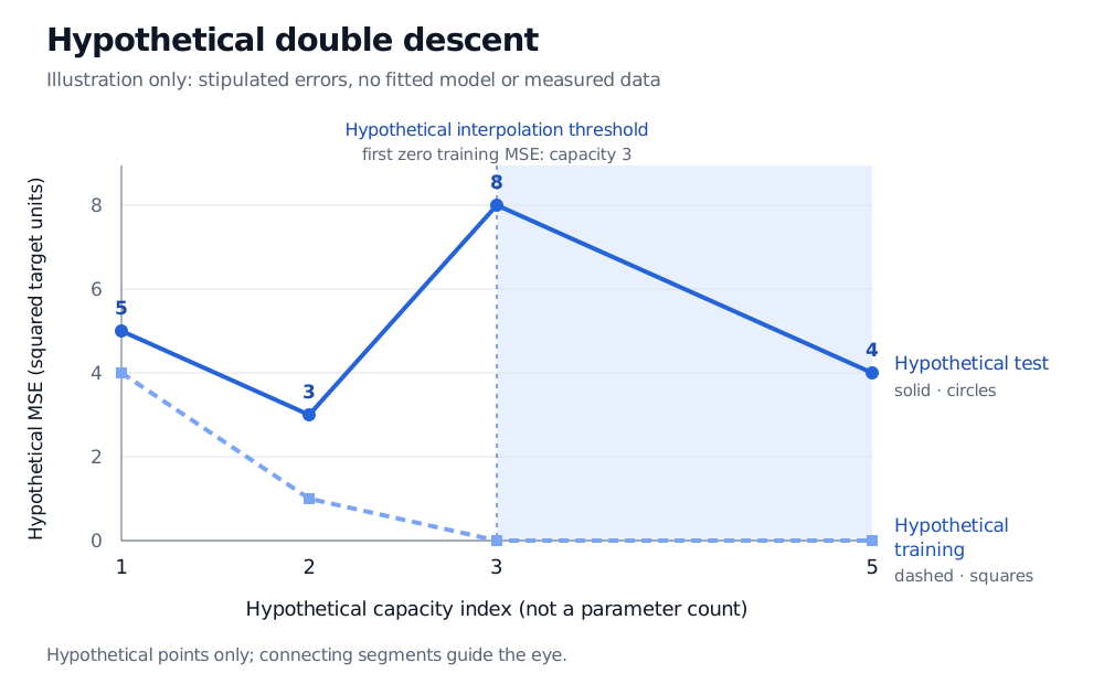
Here is a hypothetical illustration, not an experiment. The capacity index simply orders four stipulated settings; it is neither a parameter count nor a sample count. Mean squared error (MSE) uses the same squared target units throughout.
Hypothetical capacity index
Hypothetical training MSE
Hypothetical test MSE
1
4
5
2
1
3
3
0
8
5
0
4
Hypothetical illustration, not data: capacity indices 1, 2, 3 and 5 have training MSE 4, 1, 0 and 0, and test MSE 5, 3, 8 and 4, in squared target units. Training first reaches zero at 3, where test MSE peaks at 8.
Original hypothetical model-wise risk curve, not an experiment or measured data. All values are stipulated; line segments guide the eye and do not estimate intermediate errors.
The hypothetical test error first falls from 5 to 3, rises to 8 when training MSE first reaches zero at capacity 3, then falls to 4 at capacity 5. Both later settings interpolate, yet their test errors differ. Interpolation therefore does not mean perfect generalisation.
The second descent also finishes above the earlier error of 3. Even a curve with this shape need not make the largest candidate the best one. Four invented points establish no empirical result, uncertainty estimate or guarantee about the next capacity setting.
More ways to fit the same observations
Beyond interpolation, a richer class can contain many predictors that fit the training observations. Which one the algorithm selects matters. Belkin's random-feature experiments explicitly select minimum-coefficient-norm interpolants; expanding the feature class can then improve held-out performance. This is an explanation under a specified representation and fitting rule, not a promise from parameter count alone. Coefficient norm depends on the basis and its scaling.
The squared-error bias–variance identity remains valid under its assumptions. It does not require bias and variance to move monotonically with model size, or force a single U-shaped error curve.
Model-wise: vary model size while keeping the dataset and training protocol specified. This is the hypothetical figure's interpretation.
Epoch-wise: follow one architecture through training. Error can improve, worsen and improve again as training proceeds.
Sample-wise: vary training sample count for a fixed architecture and procedure. Performance can worsen over some sample-size ranges near the transition; this is not a claim that more data is generally harmful.
A sample-size learning curve and an epoch loss trace answer different questions. None of these patterns is a universal monotonicity law. Effective capacity depends on the fitting procedure as well as the architecture. Noise can accentuate a peak; explicit regularisation and early stopping can change, attenuate or hide it. Regularisation does not categorically rule double descent out.
Use validation to select, rather than predict a second dip
For a return-forecasting experiment, compare capacity, regularisation and stopping choices on development validation data. Record the training budget and compare against a simpler baseline. A peak in one historical block may reflect a particular regime or fitting instability; inspect results across suitable chronological blocks and fitting seeds.
Refit preprocessing inside each training window and respect when outcome labels become available. The time-ordered validation lesson develops that procedure (full lesson requires membership; public preview available).
Reserve the final test set for the frozen selection procedure. If a held-out error curve guides choices, it serves as validation, even when a paper or software package calls it “test error”. Continuing to enlarge or train a model until its final-test curve shows the hoped-for second descent would consume that test as selection data.