Deep kernel learning trains a neural representation through a Gaussian-process objective. See how the feature map changes similarity and why predictive uncertainty still needs validation.
Deep kernel learning
Deep kernel learning learns a neural-network transformation of the inputs together with a kernel applied to that transformation. In its standard Gaussian-process form, the network weights and kernel parameters are trained through the GP marginal likelihood. For a quant building a nonlinear regression model, this means learning which market observations should be treated as similar, rather than fixing similarity in the original feature coordinates. Wilson et al. (2016), §4 gives the defining construction.
The network changes the kernel's geometry
Write the neural feature map as ϕw and the base kernel as kθ. The effective kernel is
kdeep(x,z)=kθ(ϕw(x),ϕw(z)).
The network can bring inputs together or push them apart in feature space. A stationary base kernel can therefore produce nonstationary similarity in the original input space: equal raw displacements need not correspond to equal feature displacements. Input warping as a covariance construction is discussed in GPML, §4.2.
A minimal calculation isolates that mechanism. Take the RBF kernel with unit variance and unit length scale,
k(u,v)=exp(−2(u−v)2),
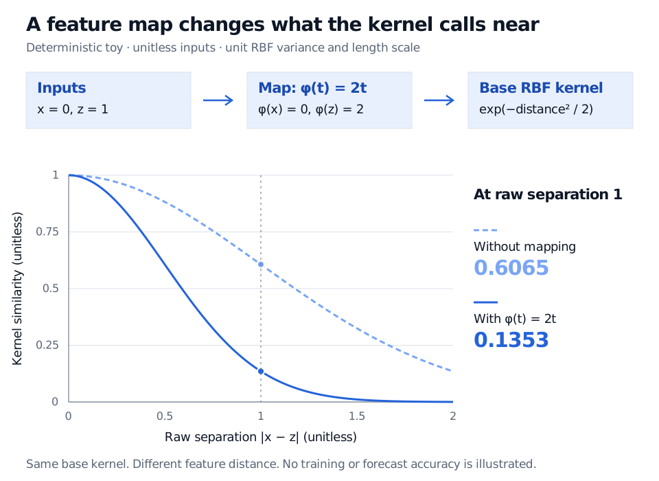
and the deterministic map ϕ(x)=2x. For the unitless inputs x=0 and z=1, the raw distance is one and the feature distance is two:
Representation supplied to the base kernel
Similarity
Raw inputs
e−1/2≈0.606531
Mapped inputs
e−2≈0.135335
Deterministic unitless scaling example. An RBF kernel with unit variance and length scale assigns inputs zero and one similarity 0.6065 without mapping and 0.1353 after mapping each input to twice its value. The mapped similarity curve decays faster with raw separation.
Original deterministic illustration, not a fitted deep network. Scaling the feature distance changes similarity while leaving the base RBF formula unchanged.
This linear map is only an arithmetic illustration; no network has been trained. Here it is equivalent to halving the RBF length scale in raw coordinates. A nonlinear learned map can make more elaborate, location-dependent changes.
Kernel validity survives the transformation. If the base kernel is valid, its Gram matrix evaluated at any transformed inputs is positive semidefinite. That is exactly the matrix produced by the composed kernel on the original inputs. For these two points the diagonal entries are one, the off-diagonal entries are e−2, and the eigenvalues are 1−e−2≈0.864665 and 1+e−2≈1.135335. Both are positive. The finite example illustrates the general Gram-matrix argument; it does not prove validity on its own. See GPML, §4.1.
What is actually learned
For zero-mean GP regression with independent Gaussian observation noise of variance σn2, let C=Kdeep+σn2I. Training maximizes
This integrates out the latent GP function values. In the usual optimization treatment, it does not integrate out the neural weights. The data-fit and log-determinant terms are coupled through the same covariance matrix; changing the representation changes both. GPML, §5.4 explains this objective.
A frozen embedding followed by a separately fitted GP also defines a composed kernel, but it lacks this joint training step. Deep kernel learning also differs from a deep GP, whose intermediate mappings are themselves stochastic GP layers. The original scalable DKL paper used structured kernel interpolation and inducing points; composing a kernel with a network alone does not make ordinary dense GP computations cheap. Wilson et al., §§2–4.
A GP output is not a calibration certificate
The predictive distribution is conditional on the fitted representation, kernel and likelihood. Uncertainty about optimized network weights is absent from that conditional distribution. Valid covariance matrices ensure a coherent model, not that its intervals achieve their nominal coverage on future observations.
Ober, Rasmussen and van der Wilk (2021) demonstrate that marginal-likelihood-trained DKL can overfit in some settings. For a financial forecasting application, assess predictive coverage on chronologically held-out data and keep feature fitting within each training window. A learned representation can map an unfamiliar market state close to training observations; raw distance alone does not ensure high predictive uncertainty.