Betting against correlation separates the correlation component of market beta from volatility. See how beta balancing changes leverage, financing and the interpretation of the factor payoff.
Betting against correlation
Betting against correlation (BAC) is an equity factor that buys stocks with lower correlation to the market and shorts stocks with higher correlation, while controlling for stock volatility and balancing the legs’ market beta. It lets a quant ask whether the low-risk effect extends to market co-movement itself, rather than merely to quiet stocks. AQR’s explanation motivates this distinction by splitting beta into its ingredients.
Which part of beta are you buying?
For returns measured on a consistent basis, market beta satisfies
βi=Var(RM)Cov(Ri,RM)=ρiMσMσi.
Here ρiM is the stock’s correlation with the market, σi is its return volatility, and σM is market volatility. Across stocks measured against the same market, the denominator is common. A low beta can therefore come from low volatility, low market correlation, or both.
A simple low-beta sort mixes those channels. BAC controls volatility to focus on correlation. The correlation is with the market, not the average pairwise correlation among the stocks in the basket. Nor is the objective to find the portfolio with minimum variance.
The original construction uses stock sorts
In Asness, Frazzini, Gormsen and Pedersen’s paper, Section 2.1, stocks are first sorted into five volatility groups within each country. Each group has low- and high-correlation portfolios, weighted using correlation ranks and rebalanced monthly. Both legs are scaled to beta one; low minus high forms that group’s BAC. Averaging the five gives national BAC. The global factor weights national factors by lagged market capitalisation.
The authors estimate correlation using five years of overlapping three-day log returns and volatility using one year of daily log returns. They shrink estimated betas toward one before setting leverage. Volatility groups control stock characteristics; they do not guarantee equal realised volatility of the resulting baskets.
This design tests leverage-constraint explanations: investors who cannot lever easily may bid up high-beta stocks. The paper’s findings support that mechanism without establishing it as the sole explanation of the low-risk effect. AQR’s research summary also describes evidence for a separate lottery-demand channel.
A two-basket calculation: beta neutral, financing required
Consider two fictional baskets with equal stipulated annual volatility of 30%, a market volatility of 20%, and positive market correlations. These are teaching inputs, not estimated stocks or a replication of the paper’s sorts and shrinkage.
Input
Low-correlation basket L
High-correlation basket H
Market correlation
0.20
0.80
Annual volatility
30%
30%
Beta, ρσ/σM
0.30
1.20
Signed risky weight
1/0.30=10/3
−1/1.20=−5/6
Contribution to market beta
+1
−1
Weights are notionals per common reference amount. The long position is about 3.333 units and the short position about 0.833 units. Consequently,
The risky positions have zero ex ante market beta, net notional 2.5, and gross exposure about 4.167 times the reference amount. They are not dollar neutral. For a portfolio with one unit of equity, the balancing cash weight is 1−2.5=−1.5: borrowing is required. Alternatively, a zero-initial-cost factor payoff uses cash weight −2.5 against the risky legs. These are different capital conventions for the same risky exposures.
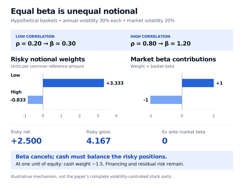
Two hypothetical baskets have annual volatility 30% with a market at 20%. Correlations 0.20 and 0.80 imply betas 0.30 and 1.20. Risky weights +3.333 and −0.833 give beta contributions +1 and −1. Risky net is +2.500, gross 4.167, and market beta zero.
Original hypothetical illustration. Equalising each leg to one unit of market beta cancels estimated market exposure while leaving substantial risky notionals and a financing requirement.
Suppose the baskets subsequently earn simple excess returns, over the same period and cash rate, of 1% and 2%. The idealised factor payoff per reference amount is
That is 1.667% of the reference amount: the leveraged long contributes 3.333% and the short subtracts 1.667%. The lower-return basket can still generate a positive spread after scaling. This arithmetic assumes borrowing and lending at Rf, with no trading costs or stock-borrow fees. The result is a payoff under a specified scaling convention; it is not a promised premium or an unqualified return on the margin capital needed to implement the trade.
What the neutral beta leaves behind
Market neutrality always needs a specified exposure measure. Estimated beta can cancel at formation while realised beta drifts as correlations and volatilities change. Even if beta remains exactly zero, residual stock risk, sector exposures and losses remain. Short-sale availability, financing spreads and margin calls can also change the implementable payoff. A beta close to zero makes inverse-beta scaling especially unstable; the example deliberately uses positive betas away from zero.
For the risk accounting behind this distinction, Sharpe’s Single-Index Model separates market variance from residual variance and shows how portfolio beta aggregates. The public page provides a preview; the full lesson requires membership.