Window dressing changes disclosed holdings near a reporting date. Trace why a winner-heavy snapshot can coexist with a loss, and how to investigate the mismatch.
Window dressing
Window dressing is changing a fund's portfolio near a reporting date to make its disclosed holdings look more attractive than the portfolio investors actually experienced over the period. A familiar version sells recent losers and buys recent winners before the holdings snapshot. For a quant analyst, the consequence is a measurement problem: the securities visible at the end need not be the securities that produced the return. Agarwal, Gay and Ling's original study examines this conflict between holdings and performance.
The term concerns the presentation motive. A purchase of a winning stock, a quarter-end trade, or an unusual disclosure does not by itself establish that motive or prove fraud. A portfolio can also change for ordinary rebalancing, revised forecasts, investor subscriptions or redemptions, risk limits, and tax management.
A winner in the report, a loss in the account
Consider a fictional, fully invested long-only fund. It starts 1 January with USD80 in A and USD20 in B. Over the period to 31 March, A returns −10% and B returns +10%. Assume no distributions, external flows, fees or trading costs, and no trades until after those returns have occurred.
Stage
A value (USD)
B value (USD)
Total value (USD)
Period start
80
20
100
After the period's returns, before trading
72
22
94
After a USD52 transfer from A to B
20
74
94
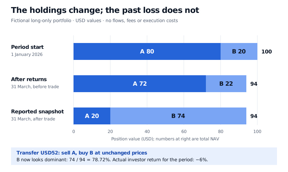
The investor's period return is 94/100−1=−6%. Immediately before the holdings snapshot, the manager sells USD52 of A and buys USD52 of B at unchanged prices. The report now shows 78.72% in B, the period's winner, because 74/94≈0.7872. This trade changes the composition of the fund, while its net asset value remains USD94 under the costless assumptions. It cannot retroactively earn B's earlier gain.
Fictional USD portfolio: start A80 and B20, total100; after returns A72 and B22, total94; after a USD52 transfer, reported A20 and B74, total94. B's reported weight is78.72%, while the actual period return remains−6%.
Original fictional ledger on a common USD scale. Prices are frozen during the final transfer; there are no flows, fees or execution costs. The report's winner-heavy appearance does not reverse the loss already incurred.
Multiplying the reported ending weights by the earlier asset returns gives a tempting number:
9420(−10%)+9474(10%)≈+5.74%.
That is an invalid attribution of this fund's realised return. It treats weights chosen after the gains and losses as though they had been in place before them. The actual beginning-weight calculation is 0.8(−10%)+0.2(10%)=−6%. Even without the final trade, price movements alone would change the weights; ending weights are generally unsuitable substitutes for beginning exposures.
Which date does the data describe?
A holdings dataset needs at least an as-of date and an availability date. The first identifies the portfolio being described. The second identifies when an outside analyst could have known about it. A later publication does not turn the snapshot into a record of everything held since the preceding report.
This matters in two different analyses. Historical performance attribution needs exposures matched to the returns they earned. A strategy that trades on disclosed holdings must wait until the disclosure was available; using the as-of date as the trading signal date creates look-ahead bias. More frequent snapshots help, but trades opened and closed between them can still disappear from view.
The incentive is also dynamic. In their 2014 explanation of their findings, Agarwal, Gay and Ling describe how performance between the snapshot and disclosure can influence whether investors interpret attractive holdings as skill and allocate more money. Subsequent flows are therefore part of the behavioural mechanism, rather than an independent stamp of manager quality. This describes the study's setting, without assuming a particular reporting delay applies to every fund today.
A diagnostic needs a counterfactual
The paper's backward holding return gap compares a hypothetical return reconstructed from the reported end-of-quarter portfolio with the actual fund return, with adjustments for expenses and trading costs. It is a proxy for a mismatch, not direct observation of intent. The deliberately incorrect ending-weight multiplication above illustrates the attribution trap; it is not a replication of the paper's full estimator.
A useful investigation asks what else could generate the pattern:
Passive drift and genuine strategy changes: separate price-driven changes from trades. A momentum strategy can deliberately buy recent winners throughout the year; winner exposure alone cannot distinguish it from presentation-driven trading.
Flows and round trips: reconcile subscriptions, redemptions and cash balances, then inspect trades around the snapshot where available. A reversal soon afterward is useful evidence, but isolated reversals can also reflect new information or liquidity needs.
Costs and coverage: reconcile fees, spreads, market impact, distributions and omitted positions before interpreting a holdings-versus-return difference. The example's sale and purchase total USD104 of gross trading despite transferring only USD52. Additional reversal trades would add further portfolio turnover and possible costs.
There is also a distinction from marking the close or portfolio pumping: those mechanisms seek to influence the prices used to value a portfolio near the close. The example here holds prices fixed and changes the names and weights in the report. The mechanisms can coexist, but changing a snapshot and changing a valuation price require different evidence.
For the accounting underneath these checks, Turnover and the Information Horizon derives passive weight drift and the trading required to reset a portfolio. A public preview is available; the full lesson requires membership.