Weight of evidence and information value: Definition & Examples

Weight of evidence (WOE) replaces a predictor's category or numerical bin with a log ratio comparing how frequently that bin occurs among two outcome classes. Information value (IV) combines the bins into a measure of separation between the two class-conditional distributions. In credit modelling, they let a quant inspect which borrower groups are associated with better or worse outcomes before fitting a scorecard. They do not, by themselves, produce default probabilities or establish that a predictor will work on future loans.

Choose the sign before reading the score

Define bad as an observed default within a specified outcome horizon and good as an observed non-default over that same horizon. The labels need a consistent observation window; a recently originated loan whose outcome is still unknown is not automatically good.

For bin $j$ , let $G_j$ and $B_j$ be its good and bad counts, with class totals $G$ and $B$ . Set

g_j=\mathbb{P}(X\in j\mid\text{good})=\frac{G_j}{G},\qquad b_j=\mathbb{P}(X\in j\mid\text{bad})=\frac{B_j}{B}.

Here the probabilities are empirical conditional shares in the development cohort. With positive shares, use

\mathrm{WOE}_j=\ln\frac{g_j}{b_j}.

This is the non-event-over-event convention in the SAS HPBIN definition, with default designated the event. Natural logarithms are used, without multiplying by 100.

A positive WOE means the bin holds a larger fraction of all goods than of all bads.
A negative WOE means the bin holds a larger fraction of all bads than of all goods.
Zero means the two class-conditional shares are equal.

Some implementations reverse the ratio. That reverses every WOE sign. Always check the outcome coding, numerator, logarithm base and any scaling before comparing reported values.

Two bins, two different questions

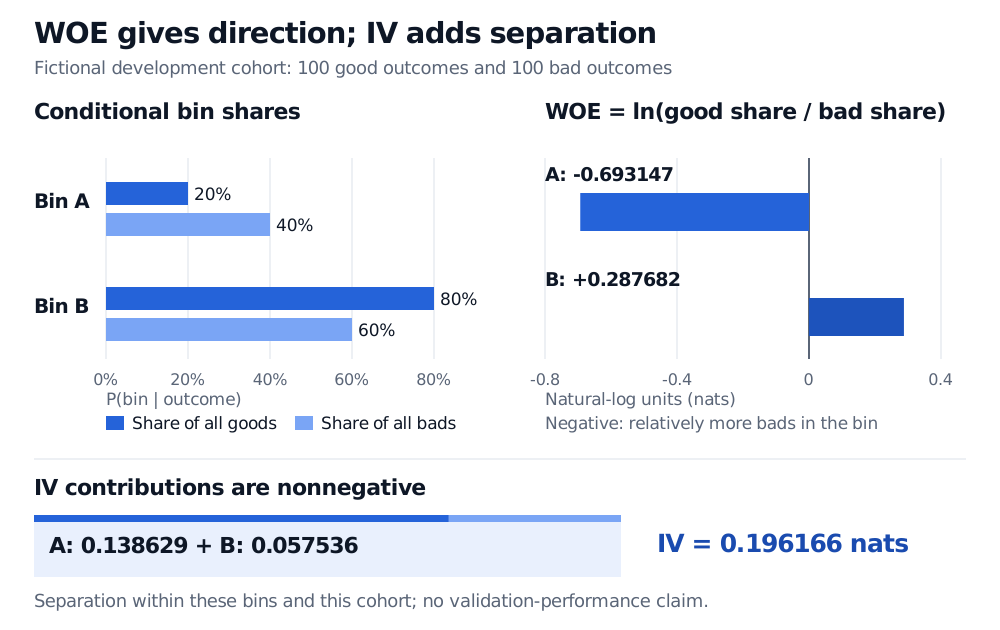
Consider a fictional development cohort containing 100 goods and 100 bads. A borrower characteristic has two bins:

Bin	Good count	Bad count	Share of all goods	Share of all bads	WOE	Observed bad rate within bin
A	20	40	0.20	0.40	−0.693147	66.67%
B	80	60	0.80	0.60	+0.287682	42.86%
Total	100	100	1.00	1.00	—	50.00%

For A, the ratio is $0.20/0.40=0.5$ , giving $\ln(0.5)=-0.693147$ . For B it is $0.80/0.60=4/3$ , giving $\ln(4/3)=0.287682$ .

The 40% bad share for A asks: “Of all bads, what fraction falls in A?” Its 66.67% bad rate asks: “Of all observations in A, what fraction is bad?” These reverse the conditioning and have different denominators. WOE uses the former kind of quantity.

Bayes' theorem connects the two. Within the same population,

\log\frac{\mathbb{P}(\text{bad}\mid X\in j)}{\mathbb{P}(\text{good}\mid X\in j)} =\log\frac{\mathbb{P}(\text{bad})}{\mathbb{P}(\text{good})}-\mathrm{WOE}_j.

Thus WOE is an adjustment to prior log-odds, rather than a probability. If the class-conditional shares stayed fixed but the overall bad rate fell to 10%, A's bad rate would become $0.1(0.4)/(0.9(0.2)+0.1(0.4))=2/11$ , or 18.18%, while its WOE would remain −0.693147. Holding those shares fixed is a stipulated scenario, not an assumption to make automatically after a population change.

A scorecard may use WOE-transformed features in logistic regression. With several correlated predictors, fitted coefficients need not equal the single-bin identity's coefficient of −1. Adding marginal WOEs is not automatically a valid joint log-odds model. The Logistic Regression and Maximum Likelihood lesson develops the binary probability model; its full teaching requires membership, with a public preview.

IV adds separation, not signed risk

For the good-over-bad convention, pair WOE with the matching difference:

\mathrm{IV}=\sum_j(g_j-b_j)\ln\frac{g_j}{b_j}.

For the fictional counts,

\begin{aligned} \mathrm{IV}_A&=(0.2-0.4)\ln(0.5)=0.1386294361,\\ \mathrm{IV}_B&=(0.8-0.6)\ln(4/3)=0.0575364145,\\ \mathrm{IV}&=0.1961658506. \end{aligned}

Fictional cohort with 100 goods and 100 bads. Bin A contains 20 percent of all goods and 40 percent of all bads, giving WOE minus 0.693147. Bin B contains 80 and 60 percent, giving plus 0.287682. IV contributions 0.138629 and 0.057536 total 0.196166 nats.

Original fictional example. WOE retains the direction of association; IV adds nonnegative contributions from both bins. Neither is a held-out performance estimate.

Each contribution is nonnegative: when $g_j-b_j$ is negative, its log ratio is also negative; when one is positive, so is the other. With strictly positive, normalised bin distributions, IV is zero exactly when the two distributions coincide. A negative result under this definition signals inconsistent signs or another calculation problem.

Expanding the sum gives

\mathrm{IV}=\sum_jg_j\ln\frac{g_j}{b_j}+\sum_jb_j\ln\frac{b_j}{g_j} =D_{\mathrm{KL}}(g\Vert b)+D_{\mathrm{KL}}(b\Vert g).

This is Jeffreys divergence, the sum of both directions of Kullback–Leibler divergence, as defined in Nielsen's discussion of statistical divergences. With natural logs its units are nats. It is not the percentage of defaults explained, and it is not mutual information between the feature and label. Reversing both the WOE ratio and the accompanying share difference leaves IV unchanged; reversing only one makes it negative.

The bins are part of the fitted model

WOE is supervised: the transformation uses outcomes. Learn bin boundaries, category merges, missing-value treatment and WOE values from training data only. When evaluating with cross-validation, repeat those fitting and feature-selection decisions inside each training fold, then apply the frozen mapping to its validation fold. The general separation of fitting from testing is explained in scikit-learn's data-leakage guidance.

For credit cohorts, the training cutoff must also respect when the outcome horizon finishes. A label eventually observed after the cutoff was not yet available at that cutoff. Predefine how an unseen category will be handled; it has no empirical training WOE of its own.

Sparse bins make extreme values easy to obtain. If one class count is zero while the other is positive, unsmoothed WOE is infinite in magnitude and the corresponding divergence contribution is infinite. If both are zero, the bin provides no observed ratio. One possible finite estimator is normalised additive smoothing across

K

retained bins:

\widetilde g_j=\frac{G_j+\alpha}{G+K\alpha},\qquad \widetilde b_j=\frac{B_j+\alpha}{B+K\alpha},\qquad \alpha>0.

Use these shares consistently in both WOE and IV. This is a stated estimator, not a claim about every package's smoothing implementation. Choose its strength using training data; smoothing does not create evidence where observations are scarce.

Finally, WOE does not itself make an ordered predictor monotonic: it assigns the measured ratio to whatever bins were chosen. Fine or outcome-optimised bins can capture sample noise. IV is a univariate, binning-dependent development statistic; it cannot measure the incremental benefit of a feature already duplicated by another predictor. Treat familiar “weak/moderate/strong” IV bands as context-dependent screening heuristics, not universal evidence. Judge the entire frozen pipeline on held-out cohorts, including probability reliability and stability through time.

Sources

SAS HPBIN: Computing the Weight of Evidence and Information Value — class-conditional count ratios and the IV sum. The article's unsmoothed definition and explicitly normalised smoothing estimator are distinguished above.
Frank Nielsen: Jensen-Shannon divergence and diversity index, §1 Origins — KL and Jeffreys divergence definitions.
scikit-learn: Common pitfalls, §12.2 Data leakage — learning transformations and feature selection within training data.

Choose the sign before reading the score

Two bins, two different questions

IV adds separation, not signed risk

The bins are part of the fitted model

Sources

Related terms

Bayes' theorem

Logistic regression fitting and SVM loss comparison