Wasserstein GAN: Definition & Examples

A Wasserstein GAN (WGAN) is a generative adversarial network that trains a generator using a critic designed to approximate the Wasserstein-1 distance between observed and generated distributions. For a quant building synthetic scenarios, it changes the distribution-matching signal; it does not certify realistic crises or correct derivative prices.

A critic measures a distribution gap

For distributions $P_r$ and $P_g$ on Euclidean space with finite first moments, Wasserstein-1 is the least expected distance needed to transport one into the other:

W_1(P_r,P_g)=\inf_{\pi\in\Pi(P_r,P_g)}\mathbb{E}_{(x,y)\sim\pi}[\lVert x-y\rVert_2].

Here $\Pi(P_r,P_g)$ contains joint distributions with those marginals. Its dual form is

W_1(P_r,P_g)=\sup_{\lVert f\rVert_{\mathrm{Lip}}\leq1}\left(\mathbb{E}_{P_r}[f(X)]-\mathbb{E}_{P_g}[f(X)]\right).

The constraint means

\lvert f(x)-f(y)\rvert\leq\lVert x-y\rVert_2

: scores cannot change faster than inputs. WGAN approximates this maximisation with a neural critic. Unlike a probability discriminator, its output is an unrestricted real score; adding a constant changes neither the gap nor the training signal. Arjovsky et al., Sections 2–3

Move half the mass, or score it

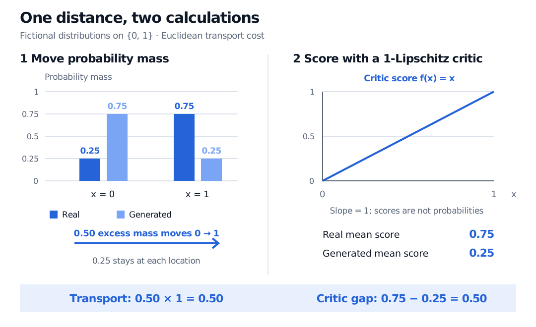
Consider a fictional binary variable taking values zero and one. The real distribution assigns probability 0.75 to one; the generated distribution assigns 0.25. These are exact population probabilities, not estimates from samples.

To turn generated mass into real mass, leave 0.25 at each location and move the remaining 0.50 from zero to one. The cost is $0.50\times1=0.50$ . No cheaper plan exists: the shortfall at one requires at least that much mass to cross the unit gap.

Now choose $f(x)=x$ , which is 1-Lipschitz. Its real mean is 0.75 and its generated mean is 0.25, so the dual gap is also 0.50. A feasible transport plan bounds the distance above, and a feasible critic bounds it below. Their equality proves $W_1=0.50$ here.

Fictional Bernoulli distributions have real mass 0.75 and generated mass 0.25 at one. Moving 0.50 mass from zero to one costs 0.50. The critic f(x) equals x and has slope one; real and generated mean scores are 0.75 and 0.25, giving the same gap of 0.50.

The transport plan and a feasible critic meet at 0.50, establishing the exact Wasserstein-1 distance for this fictional example.

Matching means alone is not generally enough. It works here because a binary distribution on these two fixed locations is determined by its probability at one. A critic restricted to linear functions could miss differences between more general distributions with equal means.

Which network minimises which loss?

Write $G_\theta(Z)$ for generated samples and $f_w$ for the critic. The ideal game is

\min_\theta\max_{\lVert f_w\rVert_{\mathrm{Lip}}\leq1}V(w,\theta),\qquad V=\mathbb{E}_{P_r}[f_w(X)]-\mathbb{E}_Z[f_w(G_\theta(Z))].

For an optimiser that performs gradient descent, use

L_C=\mathbb{E}_Z[f_w(G_\theta(Z))]-\mathbb{E}_{P_r}[f_w(X)], \qquad L_G=-\mathbb{E}_Z[f_w(G_\theta(Z))].

Freeze the generator during critic updates and the critic's parameters during generator updates, retaining derivatives through the critic to the generator. Minimising

L_C=-V

is critic ascent on

V

. Minimising

L_G

raises generated scores. Arjovsky et al., Section 3 and Algorithm 1

Clipping and gradient penalty are different approximations

Original WGAN clips critic weights to a fixed interval. For a network built from Lipschitz activations, this bounds a Lipschitz constant depending on the architecture and clipping range; it does not calibrate that constant to one. Clipping can restrict capacity and disrupt gradients.

WGAN-GP replaces clipping with a soft, two-sided penalty. In the descent convention above, its critic loss is

L_C^{\mathrm{GP}}=L_C+\lambda\mathbb{E}_{\hat X}\left[(\lVert\nabla_{\hat X}f_w(\hat X)\rVert_2-1)^2\right], \qquad \lambda>0.

It samples

\hat X=\epsilon X+(1-\epsilon)G_\theta(Z)

with independent

\epsilon\sim U[0,1]

. The generator loss remains

L_G

. This encourages gradient norm one at sampled interpolations, including penalising norms below one; the ideal constraint only requires a bound of one. A finite sampled penalty does not guarantee global 1-Lipschitz behaviour. The original GP method also omits critic batch normalisation because it couples observations, conflicting with its per-input penalty. Gulrajani et al., Sections 2–4 and Algorithm 1

The binary example makes the soft constraint concrete. Restrict the critic to $f_a(x)=ax$ with $a\geq0$ and choose $\lambda=10$ . Its penalised descent loss is $-0.5a+10(a-1)^2$ , minimised at $a=1.025$ . The raw critic gap becomes 0.5125, although the true distance remains 0.50. The penalty trades constraint violation against fit; neither this raw gap nor the penalised loss is the exact distance.

Reading a financial simulator's loss

The metric depends on the representation: distances between raw prices, standardised returns and whole paths mean different things. A change of units can change the objective's scale. Choose features and scaling for the property being modelled, and fit preprocessing on training data only.

A finite neural critic, incomplete optimisation and imperfect constraints make a logged gap a training diagnostic. It is not a universal sample-quality score. For financial paths, separately test held-out return distributions, extreme co-movements and dependence across time; a low average discrepancy does not establish accuracy in a rarely observed tail. QuantGAN concerns financial sequence generation, while WGAN specifies an adversarial objective: architecture and loss are separate choices.

For the underlying adversarial game, see Generative Adversarial Networks: Adversarial Objectives and Training Dynamics (public preview; full lesson requires membership).

Sources

Arjovsky, Chintala and Bottou — Wasserstein Generative Adversarial Networks, ICML 2017, Sections 2–3 and Algorithm 1.
Gulrajani et al. — Improved Training of Wasserstein GANs, NeurIPS 2017, Sections 2–4 and Algorithm 1.