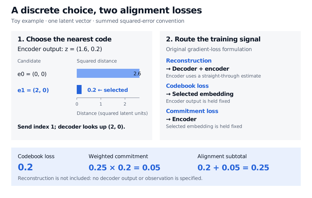
A VQ-VAE learns discrete codebook indices through nearest-vector lookup, with distinct reconstruction, codebook and commitment training signals.
Vector-quantised variational autoencoder
A vector-quantised variational autoencoder (VQ-VAE) is an autoencoder whose bottleneck replaces each continuous encoder vector with an entry from a learned codebook. The discrete representation is the entry's index; the decoder consumes its associated vector. In quant research, this offers a way to turn complex market observations into a finite vocabulary for compression or subsequent sequence modelling. Those symbols acquire economic meaning only if separate validation supports it.
What is discrete?
For encoder output ze(x) and codebook vectors e0,…,eK−1, select
The encoder output and codebook vectors remain continuous parameters. It is the index k(x) that takes finitely many values. Unlike a usual Gaussian variational autoencoder, the original VQ-VAE assigns its posterior probability to one selected index. Under its uniform training prior, the KL contribution is constant. Multiple bottleneck positions produce a sequence or grid of indices. The original paper defines this construction in Section 3.1.
A two-entry codebook
Take a toy, dimensionless encoder output ze=(1.6,0.2) with e0=(0,0) and e1=(2,0). Their squared Euclidean distances are
Choose index 1 and pass (2,0) to the decoder. Passing the unquantised (1.6,0.2) instead would bypass the discrete bottleneck.
Toy VQ-VAE: encoder output (1.6, 0.2) has squared distances 2.6 to (0, 0) and 0.2 to (2, 0), selecting index 1. Codebook loss 0.2 plus weighted commitment 0.05 gives 0.25, excluding reconstruction. The loss-routing panel distinguishes decoder, encoder and embedding updates.
The forward pass selects a code; the backward pass assigns three losses to different parameters. Distances are summed squares in toy latent units, not market returns.
Three losses, three jobs
Write the original gradient-based training objective in minimisation form:
Here sg means stop-gradient: unchanged value in the forward pass, zero derivative in the backward pass. Reconstruction trains the decoder and, through a gradient estimate, the encoder. The codebook term moves the selected embedding toward a frozen encoder output. Commitment moves the encoder output toward a frozen embedding. Exponential moving averages of assigned encoder outputs can replace gradient-based codebook updates; they do not replace reconstruction or commitment. VQ-VAE-2, Section 2.1, describes this alternative.
In the toy example, the codebook loss is 0.2. With β=0.25, weighted commitment is 0.25×0.2=0.05. Their subtotal is 0.25, excluding reconstruction: neither an observation nor a decoder output has been specified. These are sums over coordinates; averaging over the two coordinates would halve both alignment losses. Always check the reduction convention before comparing implementations.
Nearest-index selection is piecewise constant and changes abruptly at boundaries. Ordinary differentiation cannot supply the desired encoder learning signal through that selection. A common straight-through construction is
zq=ze+sg[ek−ze].
Its forward value is ek, while its backward derivative with respect to ze is the identity. Reconstruction gradients therefore reach the encoder, but do not update the embeddings through this expression. This is a surrogate gradient, not the true derivative of nearest-neighbour selection. The official Keras example's quantiser shows both stop-gradient loss terms and this construction; its losses use means rather than the toy example's coordinate sums.
A vocabulary is not yet a generator
Encoding an observed input and decoding its selected codes gives a reconstruction. To generate new samples, a model also needs a distribution over codes. The original two-stage approach fits an autoregressive generative model to encoded training examples, samples indices from that learned prior, then uses the codebook and decoder. VQ-VAE-2 extends this idea to hierarchical codes. Uniformly drawing independent entries need not reproduce the code combinations seen during training. The original paper's Section 3.3 separates representation training from prior fitting.
For a financial application, fit normalisation, encoder, codebook and prior using information available before the evaluation period. A low reconstruction loss does not establish preserved tail dependence, viable trading regimes or realistic scenario probabilities. Inspect code usage as well: a large dictionary can contain many entries that the encoder rarely selects. Finite indices provide a modelling interface, not an automatic regime taxonomy or a no-arbitrage constraint.