Value iteration is a planning algorithm that repeatedly applies a Bellman optimality update to estimates of state values. In a finite model of inventory or execution, it provides a way to compare actions using both immediate rewards and their future consequences. The computation solves the specified decision model; it does not establish that the model represents a changing market.
Turn the optimality equation into an update
Take a finite, fully observed Markov decision process with finite action sets, fixed transition probabilities , bounded expected immediate rewards and discount . Define the optimality operator by
The Bellman equation requires . Value iteration instead starts with a finite table and calculates . In a synchronous implementation, every new state value uses the same previous table. Starting from zero, is the best expected discounted reward over the next decisions, with zero continuation value afterward. This is a dynamic programming construction: solved shorter horizons supply the longer one. See Berkeley CS188 §4.3.
A state that pays repeatedly
Consider a fictional one-state model. Action A pays 1 reward unit now, B pays 0, and either action returns to the same state with certainty. The process continues forever and . Thus
| Backup count | Value | Interpretation from a zero start |
|---|---|---|
| 0 | 0 | No future decisions counted |
| 1 | 1 | One reward from A |
| 2 | 1.5 | Two discounted rewards from A |
| 3 | 1.75 | Three discounted rewards from A |
A beats B by exactly one unit for any common continuation estimate. Its infinite reward stream is , so and always choosing A is optimal. The value has not reached 2 after three backups, even though the preferred action is already correct.
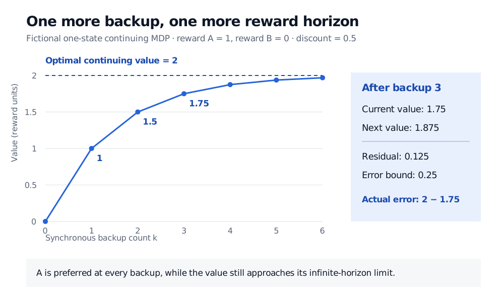
Original exact-model illustration. Each backup adds one reward horizon when starting from zero; the Bellman residual measures the remaining inconsistency, not the immediate reward.
This is a continuing state, not a terminal one. If either action instead ended the process immediately, there would be no continuation reward: A would be worth 1, not 2. A terminal state can be represented by an absorbing state paying zero thereafter, as described in Poole and Mackworth §12.5.
INTERACTIVE EXPLORER
Bellman planning and two-arm UCB
Distinguish model-based value updates from learning rewards through actions.
What convergence certifies
Under the finite discounted assumptions above, is a contraction in the maximum norm:
Here the norm is the largest absolute difference across states. Repeated synchronous updates converge from any finite initial table to the unique optimal value function. Choosing an action that maximises the backup using yields an optimal policy. The policy need not be unique: different actions can tie. MIT's Bellman notes give the contraction argument and explicitly distinguish value uniqueness from policy uniqueness.
Exact equality may require infinitely many backups. A useful stopping certificate for a current table is its Bellman residual, . The contraction gives
For the example's current value 1.75, the next backup is 1.875. The residual is 0.125; dividing by gives an error bound of 0.25, exactly the actual gap to 2. This bounds value error within the model. It is not a bound on market forecast error or, by itself, the performance loss of an extracted policy.
Updating values is not learning the environment
Asynchronous value iteration updates selected states in place using the latest table. In this discounted tabular setting, convergence requires a fair schedule that updates every state infinitely often. Repeatedly updating a convenient subset is insufficient. Sutton and Barto's §4.5 states this condition; Poole and Mackworth §12.5.2 describes the in-place variant. A single small change at one visited state is not the full-table residual used above.
Policy iteration evaluates a chosen policy and then improves it. Value iteration takes optimality backups directly. Either can serve as a planner inside model-based reinforcement learning, where the transition and reward model must first be learned. Fitting a neural value function adds approximation error; re-estimating a market model changes the operator being solved. The exact fixed-operator contraction argument does not automatically cover either case.
For a fuller finite-state treatment, the SelfMadeQuant lesson Markov Decision Processes and Value/Policy Iteration develops Bellman planning and the two solvers. Its purpose and outline are public; the full lesson requires membership.
Sources
- UC Berkeley CS188, §4.3 Value Iteration: synchronous backups, finite-horizon interpretation, contraction and policy extraction.
- Poole and Mackworth, Artificial Intelligence: Foundations of Computational Agents, §12.5: stationary decision processes, stopping states and synchronous/asynchronous value iteration.
- MIT 6.790, Value Functions and Bellman: discounted contraction and the distinction between a unique optimal value and potentially multiple optimal policies.
- Sutton and Barto, Reinforcement Learning: An Introduction, second edition in progress, copyright 2014–2015, §§4.4–4.5: value iteration and the state-revisitation condition for asynchronous updates. Section references refer to that prepublication edition.