Model-based reinforcement learning: Definition & Examples

Model-based reinforcement learning is a family of reinforcement learning methods that learn a model of an environment and use its predictions to improve a policy. For a quant studying execution, the attraction is to compare possible orders in a learned market model before incurring their real costs. The danger is that the chosen order may exploit an error in that model.

The relevant model predicts the consequences of actions: next states, rewards, or both. A neural network estimating an action's value is not, by that fact alone, an environment model. Nor does training a model-free algorithm inside a simulator automatically change that algorithm into a model-based one.

What the model adds

Suppose a state records remaining inventory, time and market observations. An environment model asks: if this order is submitted in this state, what might happen next? It may provide a distribution over outcomes or generate sampled transitions. A price forecast that ignores the order's effect does not answer the full question.

Planning uses those predicted consequences to compare actions or improve a policy. It can happen when selecting an action, or during training so that a learned policy can later act quickly. A supplied, fixed model can support planning; the distinctive learning loop here is to improve an environment model from experience and use it to improve decisions.

Sutton's original Dyna work integrates learning, planning and acting. In the simple Dyna-Q version, an observed transition both updates the model and supplies a direct Q-learning update. The model then generates hypothetical transitions for further updates. These additional updates reuse what was learned about the environment; they do not supply new independent observations.

The lesson Markov Decision Processes and Value/Policy Iteration develops the finite-state Bellman planning and model-estimation loop. Its purpose and outline are public; the full lesson requires membership.

A planner can be right about the wrong environment

For a finite next-state set, a one-step lookahead score is

\widehat Q_V(s,a)=\widehat r(s,a)+\gamma\sum_{s'}\widehat P(s'\mid s,a)V(s').

Here $\widehat r$ is the model's expected immediate reward, $\widehat P$ its transition distribution, and $V$ a supplied continuation-value estimate. The Bellman equation motivates this immediate-reward-plus-continuation structure. One backup with an arbitrary $V$ is not a claim to have found optimal action values. The discount $\gamma$ weights later rewards; it need not be a market interest-rate discount.

Consider a fictional state with two actions, A and B. There are two possible next states, called good and bad. Assign continuation values of 10 and 0 reward units and use a discount of 0.9. These values are stipulated, not learned; good and bad are continuation states, not terminal states whose later reward must be zero.

Input	A	B
Immediate reward	0	1
Model probability of good	0.8	0.6
Stipulated environment probability of good	0.4	0.6

Each bad-state probability is one minus its good-state probability. Assume the immediate rewards and continuation values are correct, so the only error is A's transition probability. Under the model,

\widehat Q_V(s,A)=0+0.9(0.8\times10+0.2\times0)=7.2,

\widehat Q_V(s,B)=1+0.9(0.6\times10+0.4\times0)=6.4.

The planner chooses A. Using the stipulated environment probabilities instead gives 3.6 for A and 6.4 for B, so B is better under the same continuation values. Choosing A sacrifices 2.8 expected reward units in this illustration. These are expected scores, not the reward from any single realised transition.

Fictional one-step planning scores in reward units. Inside the model, A scores 7.2 and B scores 6.4, so A is chosen. With the stipulated environment probabilities, A scores 3.6 and B scores 6.4, so B is chosen. Only the probability of good after A changes, from 0.8 to 0.4.

Original fictional calculation with assigned continuation values and a common scale. The model ranks actions correctly for its own probabilities, but incorrectly for the stipulated environment.

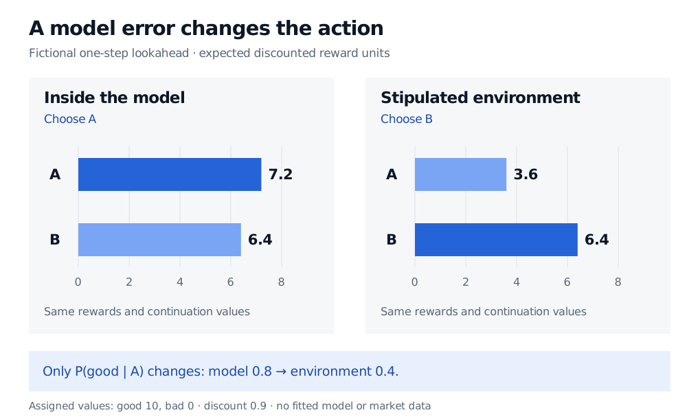
More exhaustive planning with the unchanged wrong model would not fix this ranking. It could make the planner more confident about exploiting it. This is a decision problem caused by model bias, rather than a numerical optimisation failure.

How much imagination to trust

Long simulated trajectories can compound prediction errors. A policy update can also move the agent into states and actions poorly represented in the model's training data. Low average prediction error on historical data therefore does not establish reliable values for the actions a planner will select.

Janner and co-authors' model-based policy optimisation paper studies this trade-off and uses short model-generated rollouts starting from real-data states. Its continuous-control experiments support carefully limited model use; they do not establish profitable financial trading. Short rollouts and model ensembles can help manage errors, but do not certify an accurate market simulator.

For execution research, three model choices deserve particular attention:

Action effects. Fills and market impact must depend on the proposed order. Historical replay alone does not reveal what would have happened after a different, larger order.
Changing conditions. Spread, liquidity and participant behaviour can change. A model calibrated on one period can misprice the consequences of actions in another.
The objective and constraints. Rewards should reflect the specified transaction costs, inventory risk and unfinished-order treatment. Hard position or participation limits should restrict allowed actions. An accurate transition model cannot repair a reward that rewards the wrong behaviour.

Evaluate the complete model-and-policy procedure on separate later periods using decision-time information and explicit cost assumptions, comparing it with credible simpler rules. Repeatedly adjusting the model or reward after seeing those results creates backtest overfitting. A high simulated score is evidence about the model-and-policy combination under its assumptions; it is not evidence that the model has captured every market response.

Sources

Sutton, R. S. (1990), Integrated Architectures for Learning, Planning, and Reacting Based on Approximating Dynamic Programming, ICML, pp.216–224. Original abstract read for the Dyna architecture and its integration of learned models and planning.
Sutton, R. S. and Barto, A. G., Reinforcement Learning: An Introduction, local “Second edition, in progress” text, ©2014, 2015, §§8.1–8.2, pp.195–201. Read for distribution versus sample models, planning, direct learning and the Dyna-Q loop. This is a prepublication version.
Janner, M., Fu, J., Zhang, M. and Levine, S. (2019), When to Trust Your Model: Model-Based Policy Optimization, NeurIPS, §§3–5 and §6.2. Read for model exploitation, distribution shift and short branched rollouts.
López de Prado, M. (2018), Advances in Financial Machine Learning, §§11.2–11.4. Read for historical simulation, timing, costs and selection limits. The two-action illustration and execution interpretation here are original.

What the model adds

A planner can be right about the wrong environment

How much imagination to trust

Sources

Related terms

Reinforcement learning

Transaction cost