An upper confidence bound bandit chooses actions by adding an uncertainty bonus to observed rewards. A two-arm example explains why a lower mean can win.
Upper confidence bound bandit
An upper confidence bound (UCB) bandit chooses an action by adding an uncertainty bonus to its estimated mean reward, then selecting the largest resulting score. It gives a quant researching execution choices a disciplined reason to keep testing a less observed alternative, even when another currently has the better average.
This is an approach to the multi-armed bandit problem: only the chosen action's reward is observed. The exploration is directed by uncertainty. Sutton and Barto, §2.6, contrast this with indiscriminate random exploration.
Mean plus room for improvement
Use a simple stationary model: each arm produces independent, identically distributed rewards in [0,1], with a fixed unknown mean. Rewards are observed before the next choice. Initialise by pulling each arm once.
For this article, t is the number of completed pulls. Let Ni(t) count completed pulls of arm i, and let μi(t) be their sample mean. The following UCB1-style convention selects pull t+1:
Ui(t)=μi(t)+Ni(t)2lnt,It+1∈argmaxiUi(t).
Here ln is the natural logarithm. Resolve ties by a specified rule. An untried arm must receive initial exploration rather than division by zero.
At the same t, fewer observations mean a larger bonus. If an arm is left unchosen, its count stays fixed while the logarithm grows, gradually raising its score. Once chosen, its count and mean update when the reward arrives. Sutton and Barto's discussion explains this mechanism.
The UCB1 construction comes from Auer, Cesa-Bianchi and Fischer. Time symbols differ across presentations: some index the current decision round and use counts from preceding rounds. The calculation here explicitly uses ln50 after 50 observations, choosing pull 51.
Why the lower mean wins
Imagine two fictional execution choices scored only on whether an order fills within a fixed deadline: reward 1 for success, 0 otherwise. Price, fees and adverse selection are excluded from this toy objective.
After 50 completed pulls, A has 5 successes from 10 trials; B has 22 from 40. Thus:
Arm
Completed pulls
Observed mean
Bonus
Selection score
A
10
0.50
0.8845
1.3845
B
40
0.55
0.4423
0.9923
For example,
UA(50)=0.50+102ln50≈1.384536.
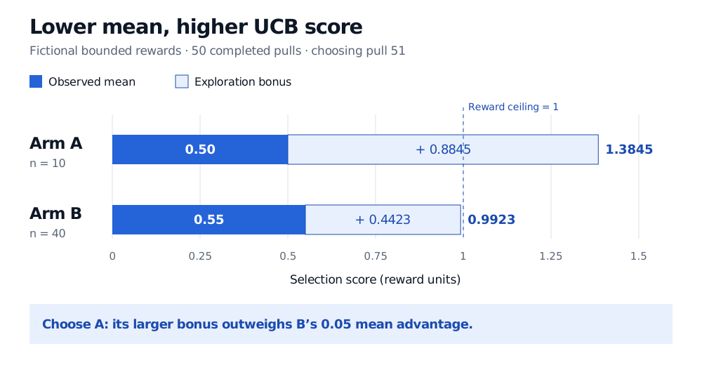
The rule chooses A for pull 51. A has one quarter of B's observations, so its bonus is twice as large. That difference outweighs B's 0.05 advantage in the observed mean. This state illustrates one decision; it is not a simulated performance comparison or a claim that A is truly better.
After 50 completed pulls, arm A has mean 0.50 and bonus 0.8845, giving score 1.3845. Arm B has mean 0.55 and bonus 0.4423, giving score 0.9923. The rule chooses A for pull 51; its score exceeds the reward ceiling of 1.
Original calculation for a fictional two-arm problem. Solid blue is the observed mean; the outlined extension is the exploration bonus. Both bars use the same reward-unit scale.
A's score exceeds 1 even though every reward is at most 1. That is permitted: the score is an optimistic selection index, not a fill probability. Clipping scores at 1 would create a different allocation rule and could introduce ties.
What the bound promises
The bonus is motivated by Hoeffding's inequality, not by a Bayesian posterior. It is not a conventional fixed 95% confidence interval. The proof must account for repeated decisions and data-dependent arm counts.
For the classical bounded stationary problem, Auer et al., Theorem 1, bound expected cumulative regret logarithmically in the horizon for fixed positive gaps between suboptimal and optimal means. Regret compares expected rewards with repeatedly choosing the best fixed arm. It does not promise the best action at every pull or a positive realised profit.
For the statistical distinction, the SelfMadeQuant lesson Confidence Intervals and Hypothesis Testing explains coverage versus posterior probability. Its preview is public; the full lesson requires membership.
Before using an execution score
A high fill rate can coexist with poor execution prices. Define the economic reward and eligible actions first; an exploration bonus supplies neither exposure limits nor a transaction-cost model. Signed, unbounded trading returns do not satisfy this bounded-reward setup merely because the same formula can be evaluated.
Markets can also change. An average over all historical fills may describe an obsolete regime. Sutton and Barto, §2.4, explain why changing problems motivate more weight on recent rewards. A windowed or discounted UCB adaptation needs its own analysis; classical regret guarantees do not automatically cover drift, constrained trading or delayed feedback. In a historical evaluation, an unfinished order's outcome is unavailable information, not an observed zero.