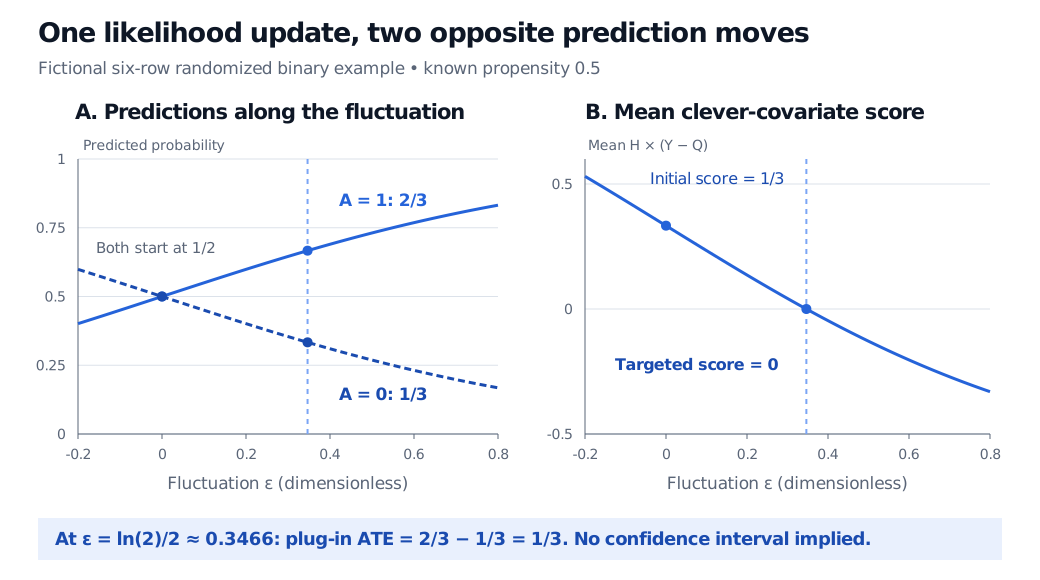
TMLE updates an initial outcome model toward a chosen estimand, then plugs the targeted predictions into that estimand. Follow a six-row logistic fluctuation and its zero score.
Targeted maximum likelihood estimation
Targeted maximum likelihood estimation (TMLE) is a framework that updates an initial statistical fit toward a specified target parameter, then evaluates that parameter using the updated fit. In quant research, the target might be the effect of a specified order-routing policy on a binary fill outcome. Accurate fill predictions alone do not guarantee an accurate policy-effect estimate: prediction loss and bias in an effect contrast are different objectives. This distinction motivates the original van der Laan–Rubin construction.
TMLE is a family of estimators. The construction below is a basic binary, single-treatment-time version for an average treatment effect.
Fix the question before targeting the fit
Observe baseline covariates W, treatment A∈{0,1} and binary outcome Y. Define
Q(a,w)=E[Y∣A=a,W=w],e(w)=P(A=1∣W=w).
Here e is the propensity score. The statistical target is
ψ=E[Q(1,W)−Q(0,W)].
A causal interpretation as E[Y(1)−Y(0)] additionally requires a well-defined intervention and consistency, conditional exchangeability given pretreatment W, and positivity in the target population: 0<e(W)<1 almost surely. The simple notation assumes no interference between units. In a routing study, order interactions or unrecorded urgency can invalidate these assumptions. Targeting cannot repair them. Gruber and van der Laan, §2, distinguish the statistical target from its causal interpretation.
The Conditional Expectation lesson develops the averaging operation used here. Its public page previews the lesson; the full lesson requires membership.
A small regression aimed at one contrast
Fit initial outcome predictions Q and obtain e from an assignment model or a known randomized design. Define the clever covariate
Fit only ϵ by Bernoulli maximum likelihood, holding the initial logit predictions fixed as an offset, with no additional intercept. Write Q∗=Qϵ. This offset-update mechanism is explained in Rosenblum and van der Laan, §1. Initial probabilities must be strictly inside (0,1) for finite logits.
At an interior optimum, the likelihood score gives
n1i∑H(Ai,Wi){Yi−Q∗(Ai,Wi)}=0.
Then average the two updated predictions over the same baseline population:
ψTMLE=n1i∑{Q∗(1,Wi)−Q∗(0,Wi)}.
This is a targeted plug-in, or substitution, estimate. For binary outcomes the fitted probabilities stay between zero and one, so their average difference stays within [−1,1]. Bounded continuous outcomes can use an appropriate rescaling and Bernoulli-type loss; arbitrary unbounded returns cannot be inserted unchanged into this binary construction. See Gruber and van der Laan, §§3.1–3.3.
Six observations: solve the fluctuation
Take six fictional independent observations from a randomized design with known e=1/2, no baseline covariates and initial predictions Q(1)=Q(0)=1/2.
Row
A
Y
H
1
1
1
2
2
1
1
2
3
1
0
2
4
0
1
−2
5
0
0
−2
6
0
0
−2
Let p=expit(2ϵ), where expit(z)=1/(1+e−z). Then Qϵ(1)=p and Qϵ(0)=1−p. Multiplying the six Bernoulli likelihood contributions gives p4(1−p)2, hence
ℓ(ϵ)=4logp+2log(1−p),ℓ′(ϵ)=8−12p.
The score vanishes at p=2/3. Moreover, ℓ′′(ϵ)=−24p(1−p)<0 at every finite ϵ, so this stationary point is the unique maximum:
ϵ=2log2≈0.3466,Q∗(1)=32,Q∗(0)=31.
The plug-in effect moves from zero to 2/3−1/3=1/3, or about 33.33 percentage points. The six values of H(Y−Q∗), in row order, are
32,32,−34,−34,32,32.
Their sum is exactly zero. Here the updated predictions also equal the two observed group proportions. That coincidence reflects this simple balanced fixture; it does not make general covariate-adjusted TMLE a raw difference of group means.
Fictional six-row example. Starting at epsilon zero, both predictions equal 1/2 and the mean clever score is 1/3. At epsilon ln(2)/2, treated prediction is 2/3, control prediction is 1/3, and the mean clever score is zero.
Original targeting paths for the six fictional observations. The fitted fluctuation sets the score to zero; it does not establish out-of-sample prediction quality or an uncertainty interval.
This example verifies the update and its score equation. Six rows do not establish asymptotic normality, confidence-interval coverage or the true population effect; no interval is inferred here.
How it relates to AIPW and prediction
Using the same H, an augmented inverse-probability-weighted (AIPW) estimate based on the initial fit is
AIPW adds a residual correction directly to an effect estimate. TMLE updates the outcome fit and then plugs it in. If AIPW instead uses the targeted fit and the targeting score is zero, its correction vanishes, giving the same estimate as TMLE. The original TMLE paper explains this estimating-equation connection. Equality with AIPW using the initial fit is not guaranteed. In this fixture it happens: the initial average correction is 1/3.
The update's in-sample likelihood improvement does not certify better held-out predictions. Predictive validation still has its own job.
A zero score is not an inference guarantee
For this target the estimated efficient influence function is
Targeting makes its empirical mean zero; it does not remove its sampling variation. Under suitable positivity, convergence and regularity conditions, double robustness permits consistency when either the outcome regression or propensity model is consistently estimated. It does not guarantee valid inference whenever one fitted model looks plausible. Rosenblum and van der Laan describe the correctly specified parametric case.
With flexible nuisance learners, standard efficient inference typically needs a negligible remainder: an appropriate product of outcome and propensity estimation errors must be op(n−1/2), alongside influence-function convergence, finite nonzero variance and control of overfitting. Cross-fitting can address own-observation overfitting; it does not supply the required convergence rates. Propensities near zero or one amplify the clever covariate, and capping them cannot create missing support. Repeated orders and shared market shocks also require dependence-aware estimation and variance theory, rather than treating every row as independent. Kennedy, §§4.1–4.3, develops the expansion, sample splitting and product-error conditions.