Structural risk minimisation selects a model class by balancing its fitted training loss against a complexity allowance. See why the best training fit can lose.
Structural risk minimisation
Structural risk minimisation (SRM) selects a prediction rule by balancing its training fit against the statistical complexity of the class it comes from. It organises candidate classes into a structure, commonly a nested hierarchy, and uses generalisation bounds to compare them. For quant research, the consequence is immediate: the model with the lowest historical prediction loss need not be the model the selection rule chooses.
Fit within a class; choose among classes
Let H1⊆H2⊆⋯ be classes of prediction rules, fixed before observing the training sample. For example, polynomial regression of degree at most one is contained in the class of degree at most two. The structure concerns sets of functions, not simply a count of coefficients.
Write RS(h) for average loss on training sample S. There are two decisions:
Within each class: empirical risk minimisation (ERM) finds a rule hj with the smallest training loss in Hj.
Across classes: SRM compares those fits using a class-dependent allowance for the gap between training and population risk.
With exact minimisation and the same loss and sample, enlarging a nested class cannot raise its minimum training loss: every earlier candidate remains available. That fact alone says nothing about the fitted rule's loss on new data. Vapnik's original overview, §IV.A, motivates SRM through this trade-off between fit and capacity. VC dimension is one capacity measure used in the theory.
A schematic selection criterion is
j∈jargmin{RS(hj)+cj}.
Here cj is a complexity allowance on the same scale as the loss. In a theorem-backed implementation, it must come from an applicable bound, with the sample size, confidence level and class complexity accounted for. Merely adding a positive number does not create a generalisation guarantee.
A lower training loss loses the comparison
Consider two synthetic nested classes, H1⊂H2, fitted for binary classification with 0–1 loss. Stipulate the following complexity charges solely to illustrate the selection arithmetic:
Class
Minimum training loss
Stipulated charge
Sum
H1
0.12
0.03
0.15
H2
0.05
0.12
0.17
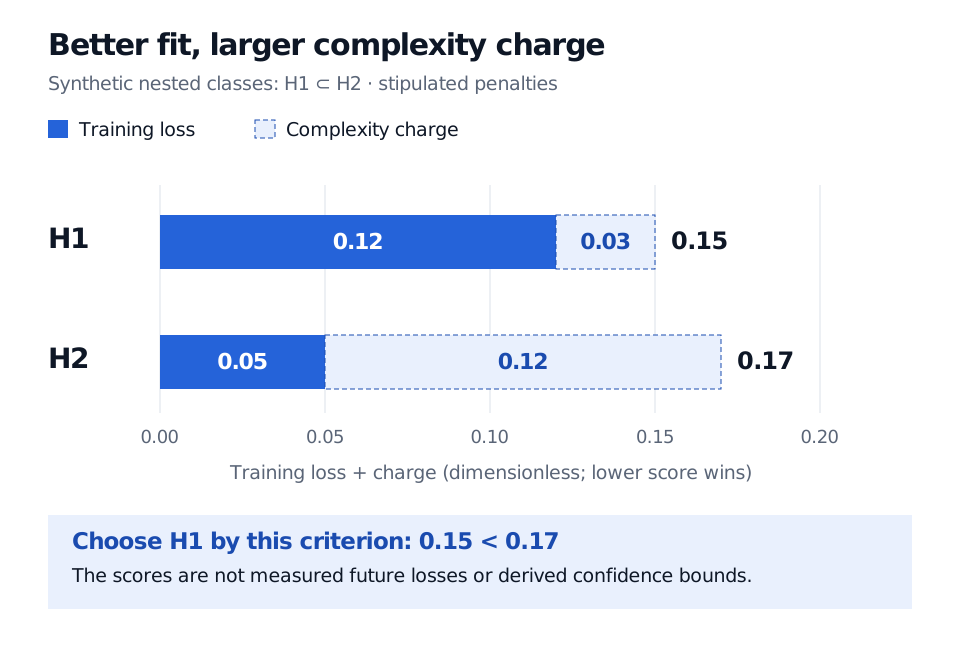
The larger class reduces training loss by 0.07, but its charge increases by 0.09. The score therefore rises by 0.02, so this criterion selects the fit from H1.
For nested classes H1 inside H2, H1 has training loss 0.12 plus stipulated complexity charge 0.03, giving score 0.15. H2 has training loss 0.05 plus charge 0.12, giving 0.17. The smaller score selects H1; the scores are not future losses or confidence bounds.
Original synthetic illustration. Both components use the same dimensionless loss scale; the complexity charges are stipulated teaching inputs, not values derived from a VC or confidence bound.
The conclusion is about the stated criterion. It does not establish that the chosen model has future error 0.15, that its true error is at most 0.15, or that it actually forecasts better than the alternative. No sampling distribution, sample size or confidence level has been supplied to justify those claims.
The guarantee must survive class selection
A bound for one class chosen in advance does not automatically retain the same confidence after searching many classes. The control must hold simultaneously over the candidate rules and the class search.
Understanding Machine Learning, §7.2, constructs SRM using uniform convergence of empirical risk. Its Theorem 7.4 allocates failure probabilities across a countable collection of classes: choose positive weights whose sum is at most one, give class j a failure allowance δj=wjδ, then use a union bound. This relies on IID sampling from one distribution and a valid uniform-convergence bound for each class. The weights and classes are specified independently of the sample. The numerical charges above are not an application of that theorem.
This also explains why a fresh round of feature engineering after seeing results needs attention: the effective search has expanded beyond the structure originally analysed.
SRM, regularisation and cross-validation
The methods are related, but the source of the selection criterion matters.
Method
What is optimised or compared?
ERM in a fixed class
Training loss over that class.
SRM
Fit plus a generalisation allowance across structured classes.
Penalised ERM
Training loss plus a penalty on the candidate rule, such as the squared coefficient norm in ridge regression.
Cross-validation
Prediction loss on observations left out of each fit.
A regularisation penalty can induce a hierarchy of constrained classes; it does not automatically equal a valid SRM confidence allowance. Cross-validation can choose a penalty strength, giving a procedure that combines penalised fitting with held-out selection. Shalizi's model-selection notes explain these connections, while Lecture 15 distinguishes fitting from held-out selection and discusses selection optimism.
For financial prediction, keep the final test set outside class design, penalty tuning and selection. Match validation to the forecast's information timing and label horizon. Overlapping return labels, serial dependence and changing market distributions can invalidate an IID bound; a complexity penalty does not repair those sampling problems. A classification-loss guarantee would also leave payoff sizes, turnover and trading costs unaddressed.
For the mathematical mechanism, the finite-class derivation in Sample Complexity Bounds shows why simultaneous control matters. For the alternative selection mechanism, the cross-validation section of Cross-Validation and Information Criteria explains held-out loss. Both full lessons require membership; public previews are available.
Sources
Vladimir N. Vapnik (1999), An Overview of Statistical Learning Theory, IEEE Transactions on Neural Networks 10(5), §IV.A, Structural Risk Minimization Induction Principle.