How much data is enough, and how much work does fitting require? Separate risk guarantees, dense-pass counts, optimisation, memory and learning-model assumptions.
Statistical and computational learning complexity
Statistical learning complexity asks how many observations are needed to attain a specified prediction-risk guarantee. Computational learning complexity asks how much computation a learner needs to attain that guarantee under a specified model of computation and data access. A quant can have enough data for a statistical argument yet miss a retraining deadline—or fit quickly without enough independent evidence that the forecast generalises.
What does “enough data” promise?
Sample complexity is meaningful only after specifying the hypothesis class, loss, sampling assumptions, accuracy and confidence. One common agnostic PAC learning target is
PS,A(LD(A(S))≤h∈HinfLD(h)+ε)≥1−δ.
Here LD is expected loss on a fresh observation from distribution D, S is the training sample, and A(S) is the fitted predictor. The probability covers the sample and any learner randomness. Accuracy ε is excess risk relative to the best predictor in the chosen class; confidence 1−δ concerns repeated training experiments. This is different from demanding absolute risk at most ε under realizability.
A sample upper bound supplies enough observations for a particular guarantee. A sample lower bound shows that fewer cannot suffice uniformly over the stated problem family and permitted learners. A sufficient bound need not be the smallest possible sample size. Ng's learning-theory notes, §§2–3, develop the IID finite-class uniform-convergence route. Those assumptions are part of the conclusion's scope: overlapping return labels and changing regimes do not become IID draws merely because a table has many rows.
What exactly is being counted?
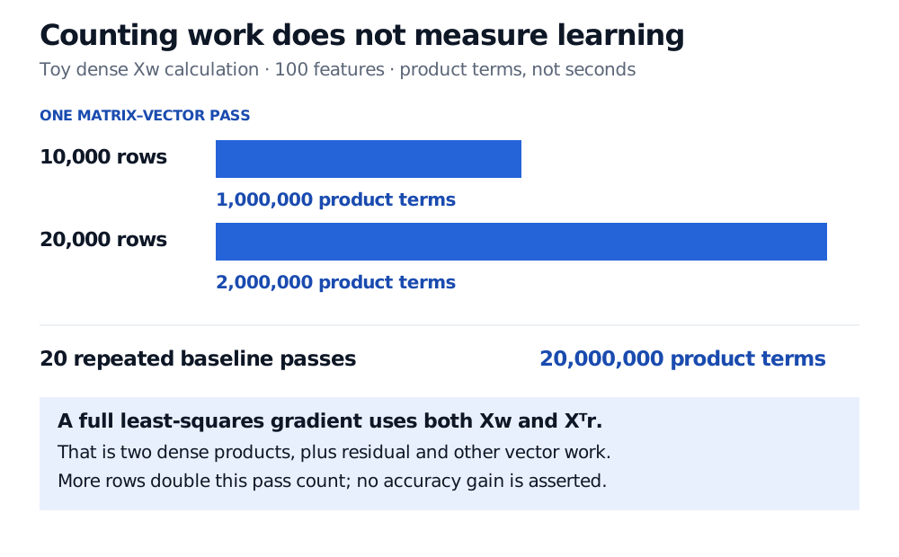
Consider a toy dense design matrix X with m=10,000 observations and p=100 feature columns, including any intercept column. Define one pass here as computing the single matrix-vector product Xw using ordinary row dot products. Each of the m rows has p product terms:
mp=10,000×100=1,000,000.
Counting each multiply-and-accumulate term as one unit, 20 such passes contain 20,000,000 product terms. Doubling the rows to 20,000, with 100 columns unchanged, gives 2,000,000 per pass. This convention counts an accumulation into a zero-initialised output; counting multiplications and additions separately uses a different unit.
Toy dense matrix-vector product with 100 features: 10,000 rows require 1,000,000 product terms per pass; 20,000 rows require 2,000,000. Twenty baseline passes require 20,000,000 terms. A full least-squares gradient uses two dense products plus vector work.
Original operation-count illustration. A pass means one dense matrix-vector product; these counts do not measure elapsed time, accuracy or a computational lower bound.
Do not read “one pass” as “one complete gradient update.” For the averaged least-squares objective
J(w)=2m1∥Xw−y∥2,r=Xw−y,∇J(w)=m1X⊤r,
a straightforward full gradient requires two dense matrix-vector products: Xw and X⊤r. At baseline size, these contribute 2,000,000 product terms per gradient evaluation, plus residual subtraction, scaling and any parameter update. Twenty gradient evaluations therefore contribute 40,000,000 dense product terms, plus that other work. Neural-network forward propagation and backpropagation have architecture-specific costs; the same one-product convention cannot stand in for their complete training step.
These are toy operation counts. They exclude feature construction, data transfer, validation and model search. They are neither a wall-clock/GPU benchmark nor a proof that no faster method exists. Doubling the data doubles this specified dense-product count; it does not guarantee a particular improvement in forecast accuracy.
Can we find the statistically good rule?
A sample guarantee can leave the search procedure abstract. Enumerating an enormous finite class may establish existence while giving an unusable fitting method. Conversely, a fast optimiser can minimise the wrong objective or search a class unable to capture the predictive relationship. Columbia's lecture, §4, distinguishes finding a consistent hypothesis from having enough observations, and explains why the allowed output representation matters.
Before interpreting a computational claim, ask:
Which representation? Must the output belong to the original class, or may the learner use a different representation? How many bits encode inputs and coefficients?
Which access? Does it read individual examples, query a statistical-query oracle, or receive exact gradients? An oracle call can hide substantial implementation cost.
Which optimisation target? How many iterations reach the stated objective tolerance, and under what smoothness, conditioning or convexity assumptions? A cheap iteration alone supplies no convergence bound.
Which memory budget? Storing the entire dense matrix requires mp scalar entries; streaming rows changes storage and access patterns. Parameter storage alone omits the dataset and working buffers.
Computational and statistical budgets can interact: allowing more examples can make efficient learning possible when a smaller sample would require more computation. Servedio's author abstract describes formal time–sample separations for particular constructed concept classes under cryptographic assumptions. That is a qualified theoretical result, not evidence that this linear-regression example is computationally hard.