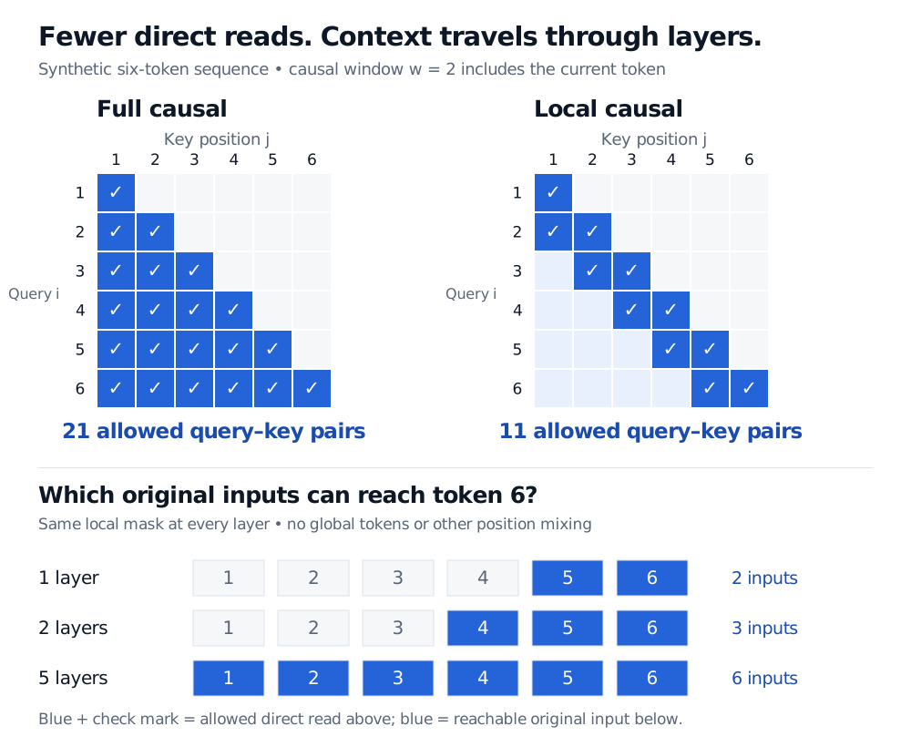
How sparse attention restricts query–key computation, with a six-token causal mask, multi-layer reach and the conditions behind linear cost.
Sparse attention
Sparse attention reduces the query–key interactions explicitly evaluated by an attention mechanism, using a restricted connectivity pattern or a selective computation rule. A quant model reading a long filing or market-event sequence can thereby spend less work on attention. The trade-off is that a useful distant disclosure may lack a direct route to the position that needs it.
Sparsity concerns connections between positions. It does not mean sparse model parameters, and small weights discovered after computing every pair do not by themselves save that computation.
Choose the available reads
For a masked scaled dot-product head, let Si be the nonempty set of key positions available to query i. Then
Here qi, kj and vj are the query, key and value vectors; dk is the key dimension. Softmax normalises over allowed keys only. Excluded positions have zero weight. Deleting weights after a full softmax without renormalising gives a different operation. Even when logits on retained edges are unchanged, removing other edges generally changes their normalised weights.
A causal local window of width w, counting the current position, uses
Si={max(1,i−w+1),…,i}.
Causality prohibits future reads; locality additionally prohibits sufficiently distant past reads. Full causal attention is still quadratic in sequence length, because its growing prefix contains many more pairs than a fixed local window.
Six tokens: count connections before claiming speed
Take six positions and w=2. Position 1 reads itself. Every later position reads itself and its immediate predecessor. The number of allowed pairs is
1+5⋅2=11,versus1+2+3+4+5+6=21
for full causal attention. These are permitted score positions for one head in one layer, not measured runtime or total model operations. In particular, position 6 directly reads only positions 5 and 6; it cannot directly select position 1's value in this layer.
Synthetic six-token causal masks have 21 full causal pairs and 11 local pairs when window width two includes the current token. Under repeated local layers, original inputs reachable at token six are five and six after one layer, four through six after two, and one through six after five.
Original connectivity example. The upper panels count direct reads; the lower panel tracks possible information paths through repeated local layers, not learned attention weights.
The local restriction need not erase every influence from older inputs. At layer two, position 6 can read position 5's layer-one representation, which may already contain information from position 4. With this same mask at every layer and no other mixing across positions, L layers permit original positions
max(1,i−L(w−1)),…,i
to reach position i. Thus five layers permit a path from original position 1 to position 6. A permitted path establishes possible dependence, not successful retention or retrieval: intervening representations and learned weights can lose the relevant detail.
Local, global and content-selected patterns
Different sparse designs choose different routes:
Local and dilated windows retain nearby positions or spaced positions. Longformer combines windowed attention with selected global tokens. In its bidirectional document encoder, global tokens read the sequence and all tokens can read them. Beltagy, Peters and Cohan, §3.1
Local, random and global connections are combined in BigBird. The additional edges provide routes between distant regions. Its expressivity results have specific architectural assumptions; they do not promise that any arbitrary sparse mask matches dense attention at the same depth or forecast accuracy. Zaheer et al., §§2–3
Content-selected neighbourhoods use the representations rather than just sequence distance. Reformer uses locality-sensitive hashing, sorting and chunks to approximate reads from similar keys, with possible misses from hash-based selection. Its reported attention scaling is O(nlogn), rather than the fixed-window rule below. Kitaev, Kaiser and Levskaya, §2
Selective queries are another form of computational sparsity. Informer's ProbSparse estimates a query-selection score from sampled query–key pairs, then evaluates selected queries against the keys. Other rows use an initial aggregate context; the paper's unmasked algorithm uses mean values, with a cumulative-sum modification for masking. This is not simply the same narrow window for every query. Zhou et al., §3 and Appendix E.2
Global reads also take layers to relay newly collected information. In a bidirectional encoder, a global token can gather an input in one layer and another token can read that updated global representation in the next. Simultaneous attention updates do not let the second token consume that newly gathered information within the same layer.
For forecasting, a global token must obey the information boundary too. A token that aggregates future observations and broadcasts that summary creates look-ahead bias, even if the ordinary tokens have local causal masks. Bidirectional processing of a completed filing already available at decision time has a different boundary. Features and publication timestamps must also respect that boundary.
When the cost is linear
For n≥w, the causal local mask has
E=nw−2w(w−1)
allowed pairs. Scoring and combining values cost O(E(dk+dv)) for key and value widths dk,dv, excluding projections and other network work. The allowed coefficient count is O(nw). Calling the attention operation linear in n holds the window, head count and feature widths fixed. Whole-stack scaling also depends on depth: increasing depth with sequence length to extend local reach adds work. Adding g global tokens introduces an additional O(ng) connection term, so g must also stay bounded for linear scaling.
These savings require an implementation that exploits the pattern. Forming the full score matrix and then applying a sparse mask still performs the full matrix multiplication. Block or band computations can skip excluded regions, but padding, indexing, kernel launches and hardware utilisation affect actual speed. The original Sparse Transformer paper, §5.5 describes block-based computation; Longformer, §3.2 compares materially different implementations of its pattern.
FlashAttention addresses a separate bottleneck: its dense form reduces memory traffic and avoids storing the full attention matrix while retaining dense attention arithmetic. Linear attention instead aggregates feature-mapped keys and values, while low-rank attention compresses the sequence axis. A lower memory requirement alone does not identify which computation or approximation a model uses.
For the underlying weighted-context formula and vector roles, the SelfMadeQuant query–key–value lesson provides the foundation (public preview; membership required for the full lesson). For a financial application, evaluate the sparse pattern's retrieval failures and forecast quality alongside measured latency on the same dated inputs. Longer feasible input is a capacity benefit, not evidence of a better trading signal.