Simpson's rule: Definition & Examples

Simpson's rule approximates a definite integral by integrating quadratic curves fitted through equally spaced samples. Its familiar weights are

1,4,2,4,\ldots,2,4,1

. Despite using quadratic pieces, it integrates every polynomial through degree three exactly.

That extra degree matters when a quant evaluates a smooth expected payoff or probability numerically: a weighted sum can deliver much more accuracy than the same grid's straight-line approximation. The gain depends on the integrand's smoothness, not on the financial label attached to the integral.

Why the middle value gets four times the weight

On one pair of subintervals, with points $a,a+h,a+2h$ , the quadratic interpolant has integral

\frac{h}{3}\left[f(a)+4f(a+h)+f(a+2h)\right].

The midpoint therefore contributes four times as much as either endpoint. Now divide

[a,b]

into an even number

n

of equal subintervals, set

h=(b-a)/n

, and write

f_i=f(a+ih)

. Adding the local integrals gives the composite formula

S_n=\frac{h}{3}\left[f_0+4\sum_{j=1}^{n/2}f_{2j-1}+2\sum_{j=1}^{n/2-1}f_{2j}+f_n\right].

The second sum is empty when $n=2$ . Shared endpoints of neighbouring quadratic pieces get weight two; the two outside endpoints retain weight one. Here $n$ counts subintervals: there are $n+1$ sample points and $n/2$ quadratic pieces. An odd number of subintervals cannot be covered by this formula without an additional rule.

Why does a quadratic construction handle cubics? For a cubic, subtracting its three-point quadratic interpolant leaves a multiple of

(x-m)((x-m)^2-h^2)

, where

m

is the middle node. That difference is odd around

m

, so its integral across the symmetric pair vanishes. Cubic exactness concerns the integral; the fitted parabola need not coincide with the cubic between samples.

The NIST Digital Library of Mathematical Functions gives both the elementary and composite formulas. Equal spacing is essential to the weights above; SciPy's documentation distinguishes their cubic exactness from quadratic exactness on irregular samples.

The first polynomial it misses

Take the dimensionless benchmark $f(x)=x^4$ on $[0,1]$ . Its exact integral is

I=\int_0^1 x^4\,dx=\frac15.

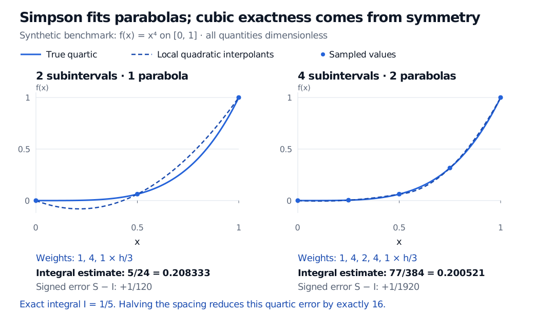
With two subintervals, the samples are $0,1/16,1$ , so

S_2=\frac16\left[0+4\left(\frac1{16}\right)+1\right]=\frac5{24}.

Refining the grid shows the characteristic fourth-order pattern:

Subintervals $n$	Simpson estimate $S_n$	Signed error $S_n-I$
$2$	$5/24\approx0.208333$	$+1/120$
$4$	$77/384\approx0.200521$	$+1/1920$
$8$	$1229/6144\approx0.200033$	$+1/30720$

Simpson interpolation of x to the fourth power on zero to one: one parabola with two subintervals gives 5/24 and error plus 1/120; two parabolas with four subintervals give 77/384 and error plus 1/1920. The coarse interpolant dips below zero.

Original synthetic benchmark. Dashed parabolas interpolate the filled sample points. The exact integral is $1/5$ ; halving the spacing reduces this quartic's error by exactly sixteen. The coarse interpolant can dip below zero even though the true function is nonnegative.

A financial reading is a synthetic claim paying $100X^4$ USD for a risk factor $X$ uniform on $[0,1]$ . Its undiscounted expected payoff is USD 20. Simpson gives USD 20.8333 with two subintervals and USD 20.0521 with four. These are integration errors under a specified toy model, not uncertainty about the model or a market valuation.

When the sixteen-fold improvement applies

If $f$ has a continuous fourth derivative on $[a,b]$ , with $a<b$ and $\lvert f^{(4)}(x)\rvert\le K_4$ , then

\lvert S_n-I\rvert\le\frac{K_4(b-a)^5}{180n^4}.

For $x^4$ on this interval, $f^{(4)}=24$ and the signed error is exactly $2/(15n^4)$ . In general, halving the spacing gives an error ratio approaching sixteen when a nonzero fourth-order leading term dominates. It is not an unconditional ratio for every function or grid. Cubic exactness, cancellation and floating-point rounding can obscure it.

In that smooth asymptotic regime,

\lvert S_{2n}-S_n\rvert/15

estimates the error magnitude of the finer result. It is an error estimate, not a general certified bound. For this quartic,

\lvert S_4-S_2\rvert/15=1/1920

exactly.

A payoff kink inside an integration interval breaks the smoothness assumption. Split at a known kink, and treat omitted tails separately when replacing an infinite domain by finite bounds. Refining the grid does not repair either an incorrect density or truncation error. If the integrand is a cash-flow rate in USD/year, multiply its weighted values by a spacing in years so the final answer is in USD.

For the finance setup behind these calculations, Root-Finding and Numerical Integration explains expectations as integrals and the trapezoid baseline. Its preview is public; the full lesson requires membership. Composite quadrature compares the local rules and their refinement behaviour.

Sources

James Stewart, Single Variable Calculus: Early Transcendentals, 6th edition, Thomson Brooks/Cole, 2008, §7.7, “Approximate Integration”: quadratic construction, composite weights and fourth-derivative error bound.
NIST, Digital Library of Mathematical Functions, §3.5(ii), “Simpson's Rule”: elementary and composite formulas and remainder terms.
SciPy, scipy.integrate.simpson: equal-spacing and irregular-spacing polynomial exactness.

Why the middle value gets four times the weight

The first polynomial it misses

When the sixteen-fold improvement applies

Sources

Related terms

Composite quadrature

Definite integral