SMO trains a support vector machine by solving constrained two-multiplier subproblems. A checked example shows why a single-coordinate update cannot move.
Sequential minimal optimisation
Sequential minimal optimisation (SMO) is an algorithm for training a support vector machine by repeatedly optimising two dual multipliers while holding the others fixed. It makes each inner optimisation small enough to solve analytically. For a quant fitting a classifier to financial features, SMO concerns how the chosen SVM is fitted; it does not introduce a new classifier or establish whether its signal predicts future returns. Fan, Chen and Lin describe this two-variable decomposition in Algorithm 1.
The constraint that makes two the minimum
Consider binary labels yi∈{−1,+1}, a free, unpenalised interceptb, and the soft-margin objective
w,bmin21∥w∥2+Ci=1∑nmax{0,1−yi(w⊤ϕ(xi)+b)}.
Here C>0 multiplies the sum, not the average, of hinge losses. The equivalent slack-variable formulation has ξi≥0 and yif(xi)≥1−ξi. With Kij=ϕ(xi)⊤ϕ(xj), its dual is the quadratic programme
These are the C-SVC conventions in LIBSVM §2.1. Replacing the loss sum with its average while retaining the same numerical C changes the problem: the equivalent average-loss coefficient is nC.
The equality comes from stationarity of the Lagrangian in b. At a feasible point, changing only αi by Δαi requires yiΔαi=0. Since yi is nonzero, the only feasible change is zero.
Free a second multiplier and the permissible changes instead satisfy
yiΔαi+yjΔαj=0.
The two box constraints cut this line down to a segment. SMO maximises the restricted quadratic along that segment. The remaining training observations still contribute to the subproblem; this is not an SVM trained on just two observations. Fixing or penalising the intercept changes the dual constraints, so the single-coordinate obstruction above belongs to the stated free-intercept formulation. The general pair subproblem appears in Fan et al., §1.
A complete pair step
Take two fictional, dimensionless feature vectors with a linear kernel:
x1=(1,0),y1=+1,x2=(0,1),y2=−1,C=2.
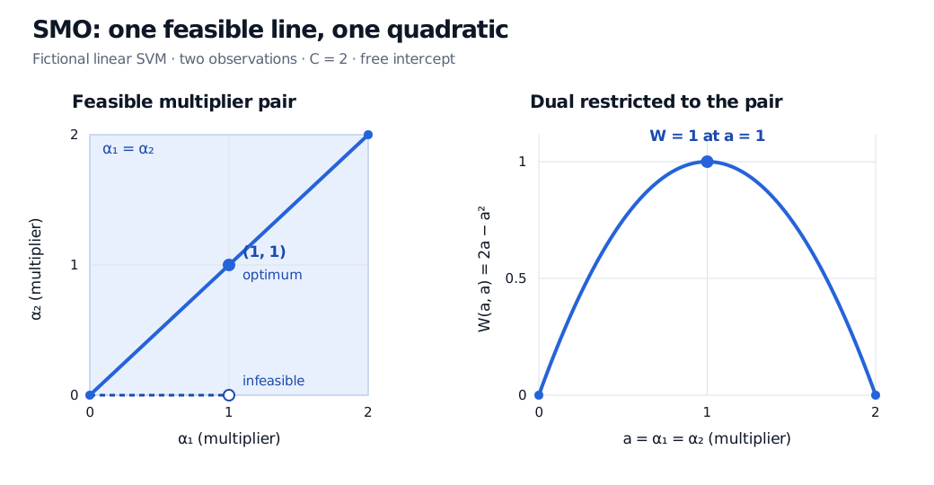
The equality is α1−α2=0. Writing both multipliers as a gives 0≤a≤2 and
W(a,a)=2a−a2=1−(a−1)2.
Starting from (0,0), the exact pair optimum is (1,1), with dual value 1. The endpoints (0,0) and (2,2) both have value 0. A move from (0,0) to (1,0) would improve the unconstrained objective, but violates the equality.
Fictional two-observation SVM with C equal to 2. Feasible multipliers lie on alpha 1 equals alpha 2 inside the square from 0 to 2. Along this line the dual value 2a minus a squared peaks at a equal to 1 with value 1.
Original deterministic example. The left panel shows the feasible pair; the right shows the objective restricted to that pair. A horizontal single-coordinate move leaves the feasible line.
Recover the primal quantities:
w=i∑αiyixi=(1,−1),b=0.
Both multipliers lie strictly between 0 and C, so both functional margins must equal one. Indeed, y1f(x1)=y2f(x2)=1. The two slack variables are zero, and the primal objective is 21(12+(−1)2)=1, matching the dual. These are functional margins; each point's geometric distance to the boundary is 1/2. A soft-margin model can have zero slack on a separable example.
What the training loop adds
With f(x)=∑kαkykK(xk,x)+b and Ei=f(xi)−yi, use
The interval [L,H] enforces both boxes and the equality. Here E1=−1, E2=1, η=2 and [L,H]=[0,2], yielding α2new=1. Reversing eta's sign requires changing the update. Zero curvature can occur with valid kernels; Platt compares endpoints instead of dividing by zero. Platt, §2.1.
The loop must also:
Choose a useful pair. Platt prioritises KKT violators and non-bound multipliers, choosing partners through error differences and fallback searches.
Update the intercept. For the +b convention, binew=b−Ei−yiΔαiKii−yjΔαjKij enforces f(xi)=yi. Use an interior multiplier's candidate, or their mean if neither is interior.
Refresh errors and repeat. Stop at the chosen KKT tolerance. Platt, §§2.2–2.5.
The Karush–Kuhn–Tucker conditions require, at an optimum,
Kernel evaluations and repeated scans can dominate runtime even though the pair solve is cheap. LIBSVM caches recently used kernel columns rather than requiring the entire dense matrix in memory. Its SMO-type solver uses later working-set selection methods, so it should not be identified with every detail of Platt's 1998 heuristic. LIBSVM §§4.1 and 5.2.
A tighter optimisation tolerance improves solution accuracy for the specified training objective. It does not repair future information in the features, choose C or the kernel, or demonstrate out-of-sample forecasting performance.
For the broader derivation, Soft-Margin SVMs and the SMO Algorithm connects the slack formulation to the dual and pairwise optimisation. The preview is public; the full lesson requires membership.