Learn how classification rules are induced, how RIPPER grows and prunes them, and why coverage, joint support and precision use different denominators.
Rule induction and RIPPER
Rule induction learns if–then rules from examples. In classification, the conditions describe a region of feature space and the conclusion predicts a class. A quant team might use a short rule list to flag potential liquidity stress: the conditions reveal which observed features trigger an alert, making the model easier to inspect and challenge.
A readable rule is still a fitted prediction. It does not establish that the conditions cause stress or that the relationship will persist.
One rule, three questions
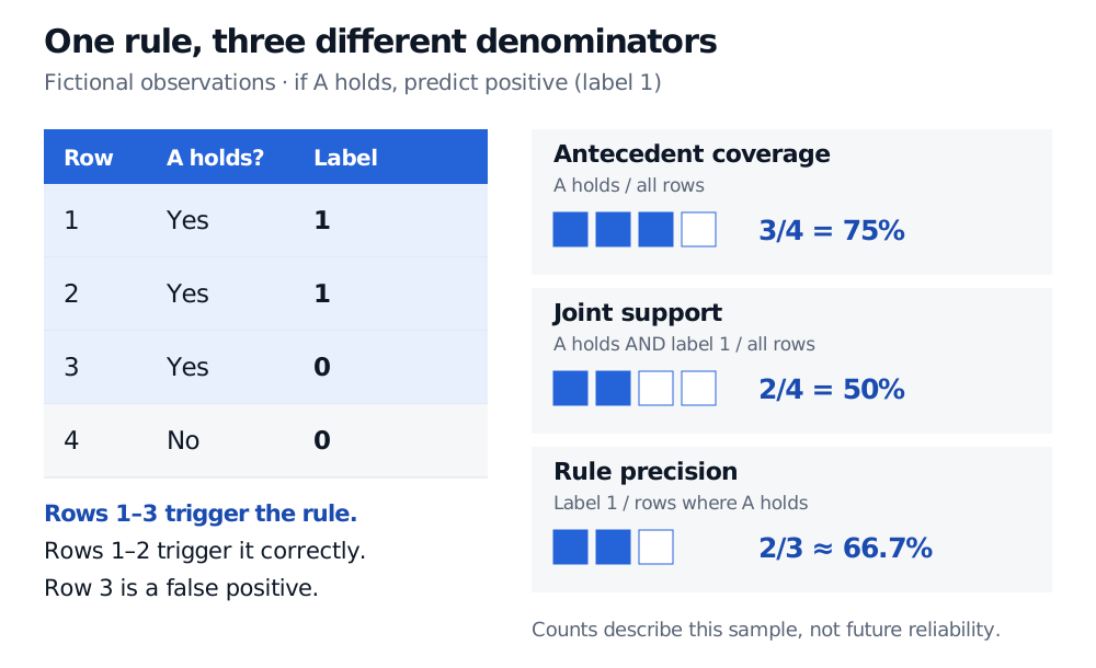
Consider four fictional observations. Condition A is a feature test available at the forecast time, such as a spread exceeding a chosen threshold. Label 1 means stress in a specified subsequent interval; label 0 means no stress. The threshold and horizon are deliberately left unspecified: this example checks counting, not a trading signal.
Observation
Condition A holds?
Observed label
1
Yes
1
2
Yes
1
3
Yes
0
4
No
0
The candidate rule is “if A holds, predict positive.” Its antecedent is A; its consequent is the positive class. Define the denominators explicitly:
Antecedent coverage: the fraction of all observations meeting A, 3/4=75%.
Joint support: the fraction meeting A and having label 1, 2/4=50%.
Rule precision: the fraction of covered observations whose label is 1, 2/3≈66.7%.
Four fictional observations: A holds on rows 1, 2 and 3, and labels are 1, 1, 0 and 0. Antecedent coverage is 3/4, joint support is 2/4, and rule precision is 2/3. Row 3 is a false positive.
Original fictional example. Each blue tile counts a numerator observation; outlined tiles complete that metric’s denominator. Precision excludes the row that does not trigger the rule.
The rule triggers three times, including one false positive. Observation 4 contributes to the coverage and joint-support denominators but never enters the precision denominator. If the complete classifier uses “otherwise predict negative,” only observation 3 is misclassified in this sample.
The word “support” needs a convention. Rule-learning reports sometimes use it for antecedent coverage or its count. Here, “joint support” always means the fraction satisfying both sides. This matches the association-rule definition in Agrawal and Srikant, §1; their confidence is the same conditional fraction as our rule precision. Some reports express support as a count instead of a fraction. Always inspect the definition before comparing numbers.
The association-mining term “confidence” is not a statistical confidence level. Nor is the observed two-thirds precision a calibrated probability for the next alert. These four rows provide no persuasive evidence of future reliability, especially if A was selected by searching the same rows.
How RIPPER learns a list
RIPPER stands for Repeated Incremental Pruning to Produce Error Reduction. William W. Cohen introduced it in 1995. It follows a separate-and-conquer approach: learn a rule, set aside the examples it covers, then search for another rule to cover remaining positives.
Its main operations are:
Grow: greedily add conditions using information gain on growing data.
Prune: remove final conditions using separate pruning data, reducing overfitting.
Build and optimise: continue constructing rules, then compare replacements and revisions using a description-length criterion that trades model complexity against unexplained errors.
Weka’s official JRip documentation describes these stages, class ordering and stopping criteria. JRip is an implementation of RIPPER with documented differences from Cohen’s original program. Its pruning scores also differ between building and optimisation; “maximise precision” alone is not a complete specification of the algorithm.
Pruning data participate in model selection. Evaluate the final rule list on additional untouched data; for forecasting, preserve time order and ensure features and training labels were available at each fitting date. Report held-out precision alongside the number of alerts and missed positives. A highly precise rule that fires rarely may miss most stress events.
Rules need execution semantics
A rule list commonly uses first match wins, followed by a default class if no rule matches. Suppose “if B, predict negative” precedes “if A, predict positive.” An observation satisfying both receives a negative prediction; reversing those rules changes it to positive. A later rule’s effective domain therefore excludes observations captured earlier. An unordered rule set instead needs an explicit conflict-resolution policy. Witten’s decision-rule notes explain why rules cannot always be read as independent facts.
A decision tree, including CART, can also be written as rules: each root-to-leaf path becomes a conjunction of tests. That representation does not make its learning procedure RIPPER. Tree growth recursively partitions regions; direct rule induction searches for individual rules and their list. Association-rule mining is different again: it searches for co-occurring attribute combinations, without requiring a designated prediction class or producing a complete classifier.
For the tree comparison, Decision Trees: Splitting Criteria and Pruning develops recursive splitting and complexity control. The full lesson requires membership; a public preview is available.
Sources
Weka, JRip official documentation: class description, building and optimisation stages, implementation differences and pruning options. Cites Cohen, Fast Effective Rule Induction, ICML 1995, pp.115–123.
Ian H. Witten, More Data Mining with Weka, Class 3, University of Waikato, 2014: lessons 3.1–3.3, especially PDF pp.6–7, 11, 15, 17 and 21–23.